Download
1 / 41
480 likes | 1.12k Views
ECEN 667 Power System Stability. Lecture 10: Synchronous Machine Models, Exciter Models. Prof. Tom Overbye Dept. of Electrical and Computer Engineering Texas A&M University, overbye@tamu.edu. Announcements. Read Chapter 4 Homework 3 is posted, due on Thursday Oct 5

E N D
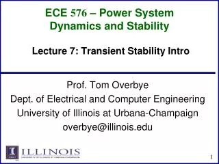
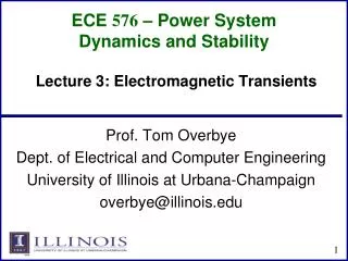
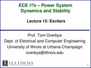
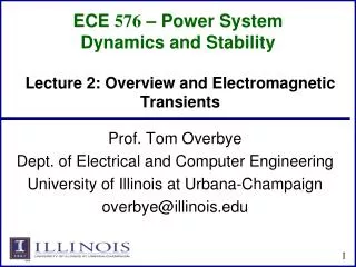
ECEN 667 Power System Stability Lecture 10: Synchronous Machine Models, Exciter Models Prof. Tom Overbye Dept. of Electrical and Computer Engineering Texas A&M University, overbye@tamu.edu
Announcements • Read Chapter 4 • Homework 3 is posted, due on Thursday Oct 5 • Midterm exam is Oct 17 in class; closed book, closed notes, one 8.5 by 11 inch hand written notesheet allowed; calculators allowed
GENSAL Block Diagram A quadratic saturation function is used. Forinitialization it only impacts the Efd value
GENSAL Example • Assume same system as before with same common generator parameters: H=3.0, D=0, Ra = 0, Xd = 2.1, Xq = 2.0, X'd = 0.3, X"d=X"q=0.2, Xl = 0.13, T'do = 7.0, T"do = 0.07, T"qo =0.07, S(1.0) =0, and S(1.2) = 0. • Same terminal conditions as before • Current of 1.0-j0.3286 and generator terminal voltage of 1.072+j0.22 = 1.0946 11.59 • Use same equation to get initial d Same delta aswith the other models
GENSAL Example • Then as beforeAnd
GENSAL Example • Giving the initial fluxes (with w = 1.0) • To get the remaining variables set the differential equations equal to zero, e.g., Solving the d-axis requires solving two linearequations for two unknowns
GENSAL Example 0.4118 Eq’=1.1298 d’=0.9614 d”=1.031 0.5882 0.17 1.8 3.460 Id=0.9909 Efd = 1.1298+1.8*0.991=2.912
Nonlinear Magnetic Circuits • Nonlinear magnetic models are needed because magnetic materials tend to saturate; that is, increasingly large amounts of current are needed to increase the flux density Linear
Saturation The fluxdensity (B)determineswhen a materialsaturates;measuredin Tesla (T)
Relative Magnetic Strength Levels • Earth’s magnetic field is between 30 and 70 mT (0.3 to 0.7 gauss) • A refrigerator magnet might have 0.005 T • A commercial neodymium magnet might be 1 T • A magnetic resonance imaging (MRI) machine would be between 1 and 3 T • Strong lab magnets can be 10 T • Frogs can be levitated at 16 T (see www.ru.nl/hfml/research/levitation/diamagnetic • A neutron star can have 1 to 100 MT!
Magnetic Saturation and Hysteresis • The below image shows the saturation curves for various materials Magnetization curves of 9 ferromagnetic materials, showing saturation. 1.Sheet steel, 2.Silicon steel, 3.Cast steel, 4.Tungsten steel, 5.Magnet steel, 6.Cast iron, 7.Nickel, 8.Cobalt, 9.Magnetite; highest saturation materials can get to around 2.2 or 2.3T H is proportional to current Image Source: en.wikipedia.org/wiki/Saturation_(magnetic)
Magnetic Saturation and Hysteresis • Magnetic materials also exhibit hysteresis, so there is some residual magnetism when the current goes to zero; design goal is to reduce the area enclosed by the hysteresis loop To minimize the amountof magnetic material,and hence cost andweight, electric machinesare designed to operateclose to saturation Image source: www.nde-ed.org/EducationResources/CommunityCollege/MagParticle/Graphics/BHCurve.gif
Saturation Models • Many different models exist to represent saturation • There is a tradeoff between accuracy and complexity • Book presents the details of fully considering saturation in Section 3.5 • One simple approach is to replace • With
Saturation Models • In steady-state this becomes • Hence saturation increases the required Efd to get a desired flux • Saturation is usually modeled using a quadratic function, with the value of Se specified at two points (often at 1.0 flux and 1.2 flux) A and B aredetermined fromthe two data points
Saturation Example • If Se = 0.1 when the flux is 1.0 and 0.5 when the flux is 1.2, what are the values of A and B using the
Saturation Example: Selection of A When selecting which of the two values of Ato use, we do not want the minimum to be between the two specified values. That is Se(1.0) and Se(1.2).
Implementing Saturation Models • When implementing saturation models in code, it is important to recognize that the function is meant to be positive, so negative values are not allowed • In large cases one is almost guaranteed to have special cases, sometimes caused by user typos • What to do if Se(1.2) < Se(1.0)? • What to do if Se(1.0) = 0 and Se(1.2) <> 0 • What to do if Se(1.0) = Se(1.2) <> 0 • Exponential saturation models have also been used
GENSAL Example with Saturation • Once E'q has been determined, the initial field current (and hence field voltage) are easily determined by recognizing in steady-state the E'qis zero Saturationcoefficientswere determinedfrom the twoinitial values Saved as case B4_GENSAL_SAT
GENROU • The GENROU model has been widely used to model round rotor machines • Saturation is assumed to occur on both the d-axis and the q-axis, making initialization slightly more difficult
GENROU Block Diagram The d-axis issimilar to thatof the GENSAL; the q-axis is nowsimilar to the d-axis. Note that saturation now affects both axes.
GENROU Initialization • Because saturation impacts both axes, the simple approach will no longer work • Key insight for determining initial d is that the magnitude of the saturation depends upon the magnitude of ", which is independent ofd • Solving for d requires an iterative approach; first get a guess of d using 3.229 from the book This point is crucial!
GENROU Initialization • Then solve five nonlinear equations for five unknowns • The five unknowns are d, E'q, E'd, 'q, and 'd • Five equations come from the terminal power flow constraints (which allow us to define d " and q" as a function of the power flow voltage, current and d) and from the differential equations initially set to zero • The d " and q" block diagram constraints • Two differential equations for the q-axis, one for the d-axis (the other equation is used to set the field voltage • Values can be determined using Newton’s method, which is needed for the nonlinear case with saturation
GENROU Initialization • Use dq transform to express terminal current as • Get expressions for "q and "d in terms of the initial terminal voltage and d • Use dq transform to express terminal voltage as • Then from These values will change during the iteration as d changes Recall Xd"=Xq"=X"and w=1 (in steady-state) Expressing complex equation as two real equations
GENROU Initialization Example • Extend the two-axis example • For two-axis assume H = 3.0 per unit-seconds, Rs=0, Xd = 2.1, Xq= 2.0, X'd= 0.3, X'q = 0.5, T'do = 7.0, T'qo = 0.75 per unit using the 100 MVA base. • For subtransient fields assume X"d=X"q=0.28, Xl = 0.13, T"do= 0.073, T"qo =0.07 • for comparison we'll initially assume no saturation • From two-axis get a guess of d
GENROU Initialization Example • And the network current and voltage in dq reference • Which gives initial subtransient fluxes (with Rs=0),
GENROU Initialization Example • Without saturation this is the exact solution • Initial values are: d = 52.1, E'q=1.1298, E'd=0.533, 'q =0.6645, and 'd=0.9614 • Efd=2.9133 Saved as case B4_GENROU_NoSat
Two-Axis versus GENROU Response Figure compares rotor angle for bus 3 fault, cleared att=1.1 seconds
GENROU with Saturation • Nonlinear approach is needed in common situation in which there is saturation • Assume previous GENROU model with S(1.0) = 0.05, and S(1.2) = 0.2. • Initial values are: d = 49.2, E'q=1.1591, E'd=0.4646, 'q =0.6146, and 'd=0.9940 • Efd=3.2186 Saved as case B4_GENROU_Sat
GENTPF and GENTPJ Models • These models were introduced into PSLF in 2009 to provide a better match between simulated and actual system results for salient pole machines • Desire was to duplicate functionality from old BPA TS code • Allows for subtransient saliency (X"d <> X"q) • Can also be used with round rotor, replacing GENSAL and GENROU • Useful reference is available at below link; includes all the equations, and saturation details https://www.wecc.biz/Reliability/gentpj-typej-definition.pdf
GENSAL Results Chief Joseph disturbance playback GENSAL BLUE = MODEL RED = ACTUAL Image source :https://www.wecc.biz/library/WECC%20Documents/Documents%20for%20Generators/Generator%20Testing%20Program/gentpj%20and%20gensal%20morel.pdf
GENTPJ Results Chief Joseph disturbance playback GENTPJ BLUE = MODEL RED = ACTUAL
GENTPF and GENTPJ Models • GENTPF/J d-axis block diagram • GENTPJ allows saturation function to include a component that depends on the stator current Most of WECC machine models are now GENTPF or GENTPJ Se = 1 + fsat( ag + Kis*It) If nonzero, Kis typically ranges from 0.02 to 0.12
Theoretical Justification for GENTPF and GENTPJ • In the GENROU and GENSAL models saturation shows up purely as an additive term of Eq’ and Ed’ • Saturation does not come into play in the network interface equations and thus with the assumption of Xq”=Xd” a simple circuit model can be used • The advantage of the GENTPF/J models is saturation really affects the entire model, and in this model it is applied to all the inductance terms simultaneously • This complicates the network boundary equations, but since these models are designed for Xq”≠ Xd” there is no increase in complexity
GENROU/GENTPJ Comparison Easy Paper Suggestion (Done by Birchfield in 2017 GM)!
GenRou, GenTPF, GenTPJ Figure compares gen 4 reactive power output for the 0.1 second fault
Exciters, Including AVR • Exciters are used to control the synchronous machine field voltage and current • Usually modeled with automatic voltage regulator included • A useful reference is IEEE Std 421.5-2016 • Just updated from the 2005 edition! • Covers the major types of exciters used in transient stability • Continuation of standard designs started with "Computer Representation of Excitation Systems," IEEE Trans. Power App. and Syst., vol. pas-87, pp. 1460-1464, June 1968 • Another reference is P. Kundur, Power System Stability and Control, EPRI, McGraw-Hill, 1994 • Exciters are covered in Chapter 8 as are block diagram basics
Functional Block Diagram Image source: Fig 8.1 of Kundur, Power System Stability and Control
Types of Exciters • None, which would be the case for a permanent magnet generator • primarily used with wind turbines with ac-dc-ac converters • DC: Utilize a dc generator as the source of the field voltage through slip rings • AC: Use an ac generator on the generator shaft, with output rectified to produce the dc field voltage; brushless with a rotating rectifier system • Static: Exciter is static, with field current supplied through slip rings