Program layers of a DBMS

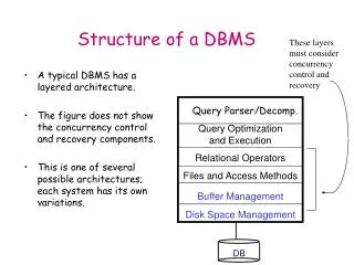
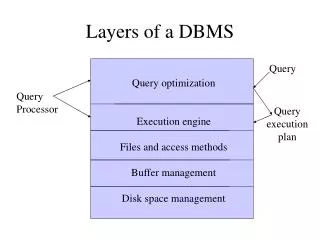
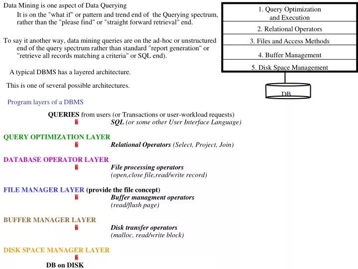
1. 1. Query Optimization and Execution 2. Relational Operators 3. Files and Access Methods 4. Buffer Management 5. Disk Space Management DB Program layers of a DBMS A typical DBMS has a layered architecture. Data Mining is one aspect of Data Querying It is on the "what if" or pattern and trend end of the Querying spectrum, rather than the "please find" or "straight forward retrieval" end. To say it another way, data mining queries are on the ad-hoc or unstructured end of the query spectrum rather than standard "report generation" or "retrieve all records matching a criteria" or SQL end). This is one of several possible architectures. QUERIES from users (or Transactions or user-workload requests) SQL (or some other User Interface Language) QUERY OPTIMIZATION LAYER Relational Operators (Select, Project, Join) DATABASE OPERATOR LAYER  File processing operators (open,closefile,read/write record) FILE MANAGER LAYER (provide the file concept)  Buffer managment operators (read/flush page) BUFFER MANAGER LAYER Disk transfer operators (malloc, read/write block) DISK SPACE MANAGER LAYER  DB on DISK

2. Data Mining Queries ARE queries and are processed (or will eventually be processed as Data Mining System mature) by a Database Management System the same way standard queries are processed today, namely: 1. SCANand PARSE (SCANNER-PARSER): A Scanner identifies the tokens or language elements of the DM query. The Parser check for syntax or grammar validity. 2. VALIDATED: The Validator checks for valid names and semantic correctness. 3. CONVERTER converts to an internal representation. |4. QUERY OPTIMIZED: the Optimzier devises a stategy for executing the DM query (chooses among alternative Query internal representations). 5. CODE GENERATION: generates code to implement each operator in the selected DM query plan (the optimizer-selected internal representation). 6. RUNTIME DATABASE PROCESSORING: run plan code. Developing new, efficient and effective DataMining Query (DMQ) processors is the central need and issue in DBMS research today (far and away!). Here we concentrate on 5, generating code (algorithms) to implement operators (at a high level) namely operators that do: Association Rule Mining, Clustering, Classification Database analysis can be broken down into 2 areas, Querying and Data Mining. Data Mining can be broken down into 2 areas, Machine Learning and Assoc. Rule Mining Machine Learning can be broken down into 2 areas, Clustering and Classification. Clustering can be broken down into [at least] 2 types, Isotropic (round clusters) and Density-based Classification can be broken down into [at least] 2 types, Model-based and Neighbor-based, though, in a real sense, even the models used are neighborhood-based: Machine Learning is almost always based on Near Neighbor Set(s), NNS. Clustering, even density based, identifies near neighbor cores 1st (round NNSs,   about a center). Classification almost always involves Near Neighbor Set voting: one decides on a set of voting neighbors who then vote on a class for the unclassified sample. Even, e.g., in Decision Tree Classification (detailed later) the training samples at the leaf of a DTC branch ARE the registered voting Near Neighbors of any unclassified sample that falls to that leaf. Classification is continuity based and Near Neighbor Sets (NNS) are the central concept in continuity >0 >0 : d(x,a)<  d(f(x),f(a))< where f assigns a class to a feature vector, or  -NNS of f(a),  a -NNS of a in its pre-image. f(Dom) categorical >0 : d(x,a)<f(x)=f(a) Next we digress temporarily into a review / development of an alternative approach to understanding data mining, using a new model called the Rolodex model.

3. name ssn lot Employee name since name dname ssn lot ssn budget lot did Employee Works_In Employee Department super-visor subor-dinate Reports_To Degree=2 relationship between entities, Employees and Departments. Must specify the “role” of each entity to distinguish them. Entity:Real-world object type distinguishable from other object types. An entity is described using a set of Attributes. Overview Review of the Entity Relationship Model Conceptual design: • What are the entities and relationships in the enterprise? • What information (attributes or features) about these entities and relationships should be stored in the database? A database `schema’ Model diagram answers these question pictorially (Entity-Relationship or ER diagrams). • Then the ER diagrams get converted to descriptive entity tables and relationship tables. Each entity set has a key. (which is the chosen identifier attribute(s) and is underlined in these notes) A Relationshipis an association among two or more entities. E.g., Employee Jonesworks inPharmacy department. Each attribute has a domain.(allowable value universe) Relationships can have attributes too! Degree=2 relationship between an entity and Itself? E.g., Employee Reports To Employee.

4. since since name name dname dname ssn ssn lot lot did did budget budget m n since name dname Employee Employee Manages Manages Department Department ssn budget lot did Works_In Employee Department 1 1 m 1 1-to-1 1-to Many Many-to-1 Many-to-Many Relationship Cardinality Constraints • (many-to-many) Works_In: An employee can work in many departments. A dept can have many employees working in it. • (1-many) e.g., Manages: • It may be required that each dept has at most 1 manager. • (1-1) Manages: In addition it may be required that each manager manages at most 1 department.

5. STUDENT COURSE S# SNAME LCODE C# CNAME SITE 25 CLAY NJ5101 8 DSDE ND 32 THAISZ NJ5102 7 CUS ND 38 GOOD FL6321 6 3UA NJ 17 BAID NY2091 5 3UA ND 57 BROWN NY2092 ENROLL LOCATION S# C# GRADE LCODE STATUS 32 8 89 NJ5101 1 32 7 91 NJ5102 1 25 7 68 FL6321 4 25 6 76 NY2091 3 32 6 62 NY2092 3 38 6 98 17 5 96 REVIEW OF HORIZONTAL DATA MODELS Once the data is modeled using, e.g., ER diagrams, a schema is defined using, e.g., the RELATIONAL DATA MODEL in which the only construct allowed is a [simple, flat] relation for both entity and relationship definition, e.g., The STUDENT and COURSE tabless represent entities. The LOCATION table represents a relationship between the LCODE and STATUS attributes (a one-to-many). The ENROLL table represents a relationshipbetween Student and Course entities (a many-to-many relationship)

6. Some Mathematical Backgound for the Rolodex Model of Data MiningThere areDUALITIESbetween each pair of:PARTITIONs,FUNCTIONs,EQUIVALENCE RELATIONsandUNDIRECTED GRAPHs Assume a Partition has uniquely labeled components (required for unambiguous reference), the Partition-inducedFunctiontakes a point to the label of its component, Function-inducedEquivalence Relationequates a pair iff they map to same value Equivalence Relation-inducedUndirected Graphhas edge for each equivalent pair, Undirected Graph-inducedPartitionis its connectivity component partition. There is aDUALITYbetween: PARTIALLY ORDERED SETsandDIRECTED ACYCLIC GRAPHs. Directed Acyclic Graph-inducedPartially Ordered Setcontains (s1,s2) iff it's an edge in graph closure Partially Ordered Set-inducedDirected Acyclic Graphcontains (s1,s2) iff it is in the POSET.

7. The RoloDex ModelA Data Cube gives a great picture of relationships, but can become gigantic (instances are bitmapped rather than listed, so there needs to be a position for each potential instance, not just for each extant instance). Bipartite, Unipartite-on-Part Experiment Gene Relationship, EGG 4 3 2 So as not to duplicate axes, this copy of G should be folded over to coincide with the other copy, producing a "conical" unipartite card. This inefficiency is especially severe in Bipartite-Unipartite-on-Part (BUP) relationships. Examples: In Bioinformatics, bipartite bipartite relationships between genes (one entity) and experiments or treatments (another entity) are studied in conjunction with unipartite relationships on genes (gene-gene or protein-protein interactions). In Market Basket Research (MBR), bipartite relationships exiting between items and customers are studied in conjunction with unipartite relationships on the customer part (or on the product part, or both). For this situation, the Relational Model provides no picture and the Data Cube Model is too inefficient (requires the unipartite relationship be redundantly replicated for every instance of the other part). Suggest the RoloDex Model. 1 G The following slide attempts to connect many such research environments (Bioinformatics, Information Retrieval (IR),Retail Association Rule Mining, (later, Collaborative Filtering (e.g., Netflix contest) is added). Does this open up new avenues for research? G 1 2 3 4 This modelling can be extended and connected together to include most entities and relationships of interest today. 1 1 3 Exp

8. 16 6 itemset itemset card 5 Item 4 3 2 1 People  Author 1 1 2 2 3 2 4 3 3 4 5 4 5 6 7 ItemSet ItemSet antecedent  Customer 1 1 1 1 1 1 1 1 5 6 16 1 1 1 1 1 1 1 1 1 Doc 1 2 3 term  G 1 2 3 4 5 6 7 Doc 4 3 2 1 PI Gene 3 4 t 5 1 6 1 2 1 3 Gene 3 Exp 4 5 6 7 Conf(AB) =Supp(AB)/Supp(A) Supp(A) = CusFreq(ItemSet) Each axis-card-axis, ac(a,b)b represents a relationship between the two axis entities. In Association Rule Mining (ARM), these are called "associations" and it is on these that ARM is done. In n ARM slide we will see that it makes no sense to try to do ARM on an entity table (axis-card pair, ac(a,b) ). On entity tables, we do Classification (CLAS). cust item card termdoc card authordoc card Most ARM interestingness measure are based on one of the [blue] supports above. In Information Retrieval, IR, the interestingness measures are: df(t) = suppG({t}, tc(t,d)); tf(t,d) is the one histogram bar in suppMG({t}, tc(t,d)) In Market Basket Research, MBR, supp(I)=suppG(I. ic(i,t)) Of course all supports are inherited redundantly by the card, c(a,b). Caution:You may have to study ARM first, then come back to this discussion of interstness measures. genegene card (ppi) docdoc People  expPI card expgene card genegene card (ppi) RoloDex Model termterm card (share stem?)

9. 16 6 itemset itemset 5 Item 4 3 2 1 Author People  1 1 2 3 2 2 3 3 4 5 4 4 5 6 7 ItemSet ItemSet antecedent  Customer, 1 1 1 1 1 1 1 1 5 6 16 1 1 1 1 1 1 1 1 1 Doc 1 2 3 term  G 1 2 3 4 5 6 7 Doc 4 3 2 1 PI Gene 3 1 4 2 term 3 5 1 4 6 1 2 1 3 Movie Gene 3 Exp 4 5 6 7 Conf(AB) =Supp(AB)/Supp(A) Supp(A) = CusFreq(ItemSet) RoloDex Model (extened futher to including Netflix data) cust item term-doc author-doc genegene (ppi) doc-doc People  Netflix ratings, dates Next, we briefly consider extensions (not yet research or studied at all by anyone - good paper topics?) of Association Rule mining to span multiple axis-card-axis situations: ac1(a,b)bc2(b,d)d and then to even longer chains. A caution: You may have to study ARM first and then come back to this. exp-gene exp-PI genegene2 (ppi) term-term (shared stem)

10. Cousin Association Rule Mining Approach (CARMA) Second Cousin Association Rules are those in which the antecedent Tset is generated by a subset of an axis which shares a card with T, which shares the card, B, with I. 2CARs can be denoted using the generating (second cousin) set or the Tset antecedent.  card (RELATIONSHIP) c(I,T) one has Association Rules among disjoint Isets, AC,  A,C I, with A∩C=∅ and Association Rulesamong disjoint Tsets, AC, A,C T, with A∩C=∅ 2 measures of AC quality: SUPP(AC) where e.g., for any Iset, A, SUPP(A) ≡ |{ t | (i,t)E iA}|CONF(AC) = SUPP(AC)/SUPP(A) First Cousin Association Rules: Given any card sharing an axis with the bipartite relationship, B(T,I), e.g., C(T,U) Cousin Association Rules: the antecedent, Tsets is generated by a subset, S, of U as follows: {tT|uS such that (t,u)C} (note this should be called an "existential first cousin AR" since we are using the existential quantifier. One can use the universal quantifier (used in MBR ARs)) E.g., S  U, A=C(S), A'T then AA' is a CAR and we can also label it SA' First Cousin Association Rules Once Removed (FCAR1Rs) are those in which both Tsets are generated by another bipartite relationship and we can label antecedent and or the consequent using the generating set or the Tset. Second Cousin Association Rules once removed are those in which the antecedent Tset is generated by a subset of an axis which shares a card with T, which shares the card, B, with I and the consequent is generated by C(T,U) (a first cousin, Tset) . 2CAR-1rs can be denoted using any combination of the generating (second cousin) set or the Tset antecedent and the generating (first cousin) or Tset consequent. Second Cousin Association Rules twice removed are those in which the antecedent Tset is generated by a subset of an axis which shares a card with T, which shares the card, B, with I and the consequent is generated by a subset of an axis which shares a card with T, which shares another first cousin card with I. 2CAR-2rs can be denoted using any combination of the generating (second cousin) set or the Tset antecedent and the generating (second cousin) or Tset consequent. Note 2CAR-2rs are also 2CAR-1rs so they can be denoted as above also. Third Cousin Association Rules are those....We note these definitions give us many opportunities to define quality measures

11. Measuring CARMA Quality in the RoloDex Model For Distance CARMA relationships, quality (e.g., supp or conf or???) can be measured using information on any/all cards along the relationship (multiple cards can contribute factors or terms or in some other way???) Item 4 3 2 1 Author People  2 1 3 2 4 3 4 5 5 6 7  Customer 1 1 1 1 1 1 1 1 1 1 1 1 1 1 1 1 1 1 1 1 1 1 1 1 1 Doc 1 2 SSR1R2 3 term  G 1 2 3 4 5 6 7 Doc 4 3 2 1 PI Gene 3 4 5 6 1 1 3 Gene Exp termdoc card authordoc card genegene card (ppi) cust item card docdoc We propose definition of Generalized Association Rules (GARs) which contains the standard "1 Entity Itemset" AR definition as a special case. Association Pathway Mining (APM) is a DM technique (application to bioinformatics?) Given Relationships, R1,R2 (RoloDex cards) with shared Entity,F, (axis), ER1FR2Gand given AE and CG, AC is a Generalized F Association Rule, with SupportR1R2(AC) = | {tE2 | aA, (a,t)R1 and cC, (c,t)R2} | ConfidenceR1R2(AC) = SupportR1R2(AC) / SupportR1(A) where as always, SupportR1(A) = |{tF|aA, (a,t)R1}|. E=G, the GAR is a standard AR iff AC=. Association Pathway Mining (APM) is the identification and assessment (e.g., support, confidence, etc.)of chains of GARs in a RoloDex.Restricting to mining cousin GARs reduces the number of strong rules or pathways links. People  expPI card expgene card t 1 2 3 genegene card (ppi) termterm card (share stem?) 4 5 6 7 More generally, for entities E, F, G and relationships, R1(E,F) and R2(F,G), A  ER1FR2G CSupport-SetR1R2(A,C) = SSR1,R2(A,C) = {tE2|aA (a,t)R1,cC (c,t)R2}. If E2 has real labels, Label-Weighted-SupportR1R2(A,C) = LWSR1R2(A,C) =tSSR1R2label(t) (un-generalized case occurs when all weights are 1) Downward closure property of Support Sets: SS(A‘,C')  SS(A,C) A'A, C'C. Therefore, if all labels are non-negative, then LWS(A,C)  LWS(A‘,C') (in order for LSW(A,C) to exceed a threshold is that all LWS(A‘,C') exceed that threshold A'A, C'C). So an Apriori-like frequent set pair mine would go as: Start with pairs of 1-sets (in E and G). The only candidate 2-antecedents with 1-consequents (equiv, 2-consequents with 1-antecedents) would be those formed by joining ... The weighted support concept can be extended to the case there R1 and/or R2 have labels as well. Vertical methods can be applied by converting F to vertical format (F instances are rows and features from other cards/axes are "rolled over" to F as derived feature attributes l2,3 l2,2 F R3 R1 G E A C

12. SOME FINAL THOUGHTS: We conclude this lecture with a short (and preliminary) discussion of where ARM, CLAS and CLUS fit with respect to entities and relationships. Please note again that you may have to come back to this after you have studied ARM, CLAS and CLUS for it to be accessible to you. A Relational Database table is a relationship (originally called a "relation" by the inventor, Codd): R(A1, ... , An) is an n-arry relationship among the columns or attributes, A1, ... , An . R is a predicate on the Cartesian product, A1  ...  An namely, P: (a1, ... , an)  R For ARM, we take 2 of the entities (attributes or columns), AT and AI (we will call the ARM entities) and a predicate on the other entities, P(true/false), so that we end up with a ternary (3 column) table for ARM, R'( AT, AI, P(1/0) ): ATAIP T1 i1 1 T1 i2 0 ... This can be projected (without loosing any information) to R" = R'P=1[AT, AI] (selection of only the "true" R'-tuples (P=1) followed by projection onto (AT, AI). Then we view each ARM-entity as a Rolodex axis and R" is the relating Rolodex card. As you will see in the ARM lectures, ARM is done on associations between the two ARM-entities. In ARM we look for associations with "strong" properties, in particular, we are interested in knowing when two disjoint sets, B and D, of one entity (e.g., AI) generate any interesing rules, BD, where the rule is interesting if, among other things, its support set, suppset(BD)={tAT | t is associated with every i in both B and D}, is a large set. More generally, suppset(A) for any subset, A, of AI is {tAT | t is associated with every i in A}. Let AI={ak | kK} then suppset(AI) = kKsuppset{ak} Clearly, if f:ATAI is a functional dependency (review in the next few slides), then suppset{ak} = f-1{ak} but these pre-image sets partition AT, so suppset(BD) will be empty unless it is a singleton set and if it is singleton, no rules can be formed from it anyway. Similar analysis will lead to the conclusion: if f:AIAT is a functional dependency, then no ARM is possible either. Therefore we can conlcude that the only ARM entities that make sense, assuming Boyce-Codd Normal Form (see next slides), are those in which (AT, AI) is [part of] a candidate key, that is, (AT, AI) is a relationship similar to Student-Course and not just a key-feature relationship such as Student-Student_name). What can be done on functional dependent pairs? Classification!