Download
1 / 36
360 likes | 367 Views
This text discusses hypothesis testing and confidence intervals for the variance of a normal population using the chi-square distribution. It also covers inference on a population proportion using the normal approximation to the binomial distribution.

E N D
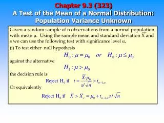
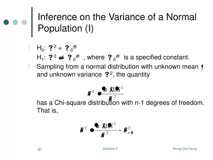
Inference on the Variance of a Normal Population (I) • H0: s2 = s02 H1: s2 s02 , where s02 is a specified constant. • Sampling from a normal distribution with unknown mean m and unknown variance s2, the quantity has a Chi-square distribution with n-1 degrees of freedom. That is, Statistics II
Inference on the Variance of a Normal Population (II) • Let X1, X2, …, Xn be a random sample for a normal distribution with unknown mean m and unknown variance s2. To test the hypothesis H0: s2 = s02 H1: s2 s02 , where s02 is a specified constant. We use the statistic • If H0 is true, then the statistic has a chi-square distribution with n-1 d.f.. Statistics II
The Reasoning • For H0 to be true, the value of 02 can not be too large or too small. • What values of 02 should we reject H0? (based on a value) What values of 02 should we conclude that there is not enough evidence to reject H0? Statistics II
Example 8-11 An automatic filling machine is used to fill bottles with liquid detergent. A random sample of 20 bottles results in a sample variance of fill volume of s2 = 0.0153 (fluid ounces)2. If the variance of fill volume exceeds 0.01 (fluid ounces)2, an unacceptable proportion of bottles will be underfilled and overfilled. Is there evidence in the sample data to suggest that the manufacturer has a problem with underfilled and overfilled bottles? Use a = 0.05, and assume that fill volume has a normal distribution. Statistics II
Hypothesis Testing on Variance - Normal Population Statistics II
Finding P-Values • Steps: 1. Find the degrees of freedom (k = n-1)in the the 2-table. 2. Compare 02 to the values in that row and find the closest one. 3. Look the a value associated with the one you pick. The p-value of your test is equal to this a value. • In example 8-11, 02 = 29.07, k = n-1 = 19, 0.05 < P-Value < 0.10 because the 2 value associated with (k = 19, a = 0.10) is 27.20 while the 2 value associated with (k = 19, a = 0.05) is 30.14 Statistics II
P-Values of Hypothesis Testing on Variance Statistics II
The Operating Characteristic Curves- Chi-square test • Use to performing sample size or type II error calculations. • The parameter l is defined as: for various sample sizes n, where s denotes the true value of the standard deviation. • Chart VI I,j,k,l are used in chi-square test. (pp. A16-A17) Statistics II
Example 8-12 Statistics II
Construction of the C.I. on the Variance • In general, the distribution of is chi-square with n-1 d.f. • Use the properties of t with n-1 d.f., Statistics II
Formula for C.I. on the Variance Statistics II
Formula for C.I. on the Variance- One-sided Statistics II
Example 8-13 Reconsider the bottle filling machine problem in Example 8-11. Find a 95% upper-C.I. on the variance? • N = 20, s2 = 0.0153 Therefore, s2 (20-1)0.0153/10.117 = 0.0287 The 95% upper-C.I. on the variance is 0.0287. In addition, the 95% upper-C.I. on the standard deviation is 0.0287 = 0.17. Statistics II
Inference on a Population Proportion(I) • H0: p = p0 H1: p p0 , where p0 is a specified constant. • P = X/n, in which X is a binomial variable, i.e., the number of success in n trials. E(X) = np, V(X) = npq = np(1-p) • If H0 is true, then using the normal approximation to the binomial, the quantity follows the standard normal distribution(Z). Statistics II
Inference on a Population Proportion (II) • Let x be the number of observations in a random sample of size n that belongs to the class associated with p. To test the hypothesis H0: p = p0 H1: p p0 , where p0 is a specified constant. We use the statistic Statistics II
The Reasoning • For H0 to be true, the value of Z0 can not be too large or too small. • What values of Z0 should we reject H0? (based on a value) What values of Z0 should we conclude that there is not enough evidence to reject H0? Statistics II
Example 8-14 A semiconductor manufacturing produces controllers used in automobile engine applications. The customer erquires that the process fallout or fraction defective at a critical manufacturing step not exceed 0.05 and that the manufacturing demonstrate process capacity at this level of quality using a = 0.05. The semiconductor manufacturer takes a random sample of 200 devices and finds that four of them are defective. Can the manufacturer demonstrate process capacity for the customer? Statistics II
The parameter of interest is the process fraction defective. • H0: p = 0.05 H1: p < 0.05 This formulation of the problem will allow the manufacturer to make a strong claim about process capacity if the null hypothesis H0: p = 0.05 is rejected. • a = 0.05, x = 4, n = 200, and p0 = 0.05. • To reject H0: p = 0.05, the test statistic Z0 must be less than -z0.05 = -1.645 • Conclusion: Since Z0 = -1.95 < -z0.05 = -1.645, we reject H0 and conclude that the process fraction defective p is less than 0.05. The P-value for this value of the test statistic Z0 is P = 0.0256, which is less than a = 0.05. We conclude that the process is capable. Statistics II
Hypothesis Testing on a Population Proportion Statistics II
P-Values of Hypothesis Testing on a Population Proportion Statistics II
How to calculate Type II Error? (I)(H0: p = p0 Vs. H1: p p0) • Under the circumstance of type II error, H0 is false. Supposed that the true value of the population proportion is p. The distribution of Z0 is: Statistics II
How to calculate Type II Error? (II) - refer to section &4.3 (&8.1) • Type II error occurred when (fail to reject H0 while H0 is false) • Therefore, Statistics II
Formula for Type II Error • Two-sided alternative H1: p p0 • One-sided alternative H1: p < p0 • One-sided alternative H1: p > p0 Statistics II
The Sample Size (I) • Given values of a and p, find the required sample size n to achieve a particular level of b. Statistics II
The Sample Size (II) • Two-sided Hypothesis Testing • One-sided Hypothesis Testing Statistics II
Example 8-15 (1) Consider the semiconductor manufacturer from Example 8-14. Suppose that his process fallout is really p = 0.03. What is the b-error for his test of process capacity, which uses n = 200 and a = 0.05? (2) Suppose that the semiconductor manuafcturer was willing to accept a b-error as large as 0.10 if the true value of the process fraction defective was p = 0.03. If the manufacturer continue to use a = 0.05, what sample size would be required? Statistics II
(1) Since H1: p < 0.05, therefore (2) The sample size required for this one-sided alternative is Statistics II
Formula for C.I. on the Population Proportion Statistics II
Formula for One-Sided C.I. on the Population Proportion Statistics II
Example 8-16 In a random sample of 85 automobile engine crankshaft bearings, 10 have a surface finish that is rougher than the specifications allow. Construct a 95% C.I. on the population proportion p? Sol: Statistics II
Choice of Sample Size for C.I. on a Population Proportion • where E is the half-width of the C.I. • Since the max value for p(1-p) is 0.25 for 0 p 1, we can use the following formula instead. Statistics II