Download
1 / 28
280 likes | 379 Views
Landcover-Dependent Fusion of SRTM Data and Airborne LIDAR Data. This work was supported by NIMA and NASA. Introduction: DEMs for Hydrologic Modeling. Goals Improve Digital Elevation Models (DEMs) for hydrologic modeling

E N D
Landcover-Dependent Fusion of SRTM Data and Airborne LIDAR Data This work was supported by NIMA and NASA
Introduction: DEMs for Hydrologic Modeling • Goals • Improve Digital Elevation Models (DEMs) for hydrologic modeling • Runoff, flood-risk assessment, and transport of non-point source pollution and sediment • Develop capability for mapping and updating topography using multiple sensors • Difficulties • Resolution/Coverage tradeoffs: DEMs with sufficient coverage often have insufficient resolution [Pickup and Marks, 2001] • Medium resolution DEMs can be derived from airborne Interferometric Synthetic Aperture Radar (INSAR) sensors but data dropouts are common • High resolution DEMs can be derived from laser altimetry (LIDAR) sensors but coverage is limited • Multi-sensor acquisitions have different extents, resolutions, and measurement errors • Approaches • Application partitioning [Pickup and Marks, 2001] • Large-scale mosaics of high-resolution DEMs [Gibeaut, Gutierrez, Smyth, Crawford, Slatton, and Neuenschwander, 1999] • Fuse DEMs acquired from multiple sensors [Slatton, Crawford, Evans, 2001]
Introduction: Data Fusion Approaches • Goals • Smooth noisy INSAR data • Combine data using formal mathematical framework to account for process dynamics and measurement errors • Potential approaches • Wavelet denoising • Provides multiresolution analysis and local smoothing, but • Not suited to multiple input/multiple output (MIMO) models • Not suited to indirect measurements • Weighted least squares estimation • Not robust to data dropouts • Stochastic process variability ignored • Multiscale Kalman filter • Allows multiresolution analysis and MMSE smoothing • Handles MIMO models • Handles indirect measurements • Provides error measure automatically .. .. ..
Outline • Introduction • Data fusion methodology • Kalman filter for data fusion • Multiscale Kalman smoother • Results • Conclusions
State Space Dynamic Model • Use state-space approach • Can model any random process having rational spectral density function with finite state dimension applicable to a large class of problems • Can estimate internal variables not directly observed [block diagram] • Able to track non-stationary and sparse data • Use discrete formulation • Data from sampled (imaged) continuous process • w and v assumed uncorrelated and have vector valued autocorrelations of a white noise sequence
input output Kalman Filter Algorithm • Kalman filter is widely used to estimate stochastic signals • Linear, time-varying filter • Implemented in time domain by a recursive algorithm • Requires prior model for filter parameters {F, Q, H, R} • Bounded estimate error covariance Pk|k • Reach steady state if {F, H} are constant and {w, v} are WSS
Multiscale Data Fusion • Motivation • Captures multiscale character of natural processes or signals • Combines signals or measurements having different resolutions • Various methods • Fine-to-coarse transformations of spatial models • Direct modeling on multiscale data structures, e.g. quadtree [MKS model] [Chou, Willsky, & Benveniste, 1994] • Multiscale signal modeling has been studied extensively in recent years Fill in all data dropouts Merge data of different resolutions INSAR LIDAR • Multiscale Kalman Smoother (MKS) algorithm • Use fractional Brownian motion data model for self-similar processes like topography[Fieguth, Karl, Willsky, & Wunsch, 1995][stochastic data model]
INSAR and LIDAR Imaging • INSAR (nominal) • Side-looking • Single-pass interferometry • Space-based • Fixed illumination • C-band - 6 cm wavelength • RMS vertical accuracy ~10 m • 30 m pixel spacing • Tens of km-scale swaths NASA Shuttle Radar Topography Mission (SRTM) imaging swath >>10 km Large coverage area: primary sensor UT LIDAR (Optech ALTM) • LIDAR (nominal) • Downward-looking • Airborne • Scanning illumination • 1 mm wavelength • RMS vertical accuracy ≥ 0.1 m • 1-5 m pixel spacing (gridded) • cm-scale footprint complementary sensor
zg < zS < zv Measuring Topography with INSAR • Problem: no direct measurement of zg in presence of vegetation • INSAR data provide height of phase scattering center zS • Cannot distinguish surface elevation zg from vegetation elevation zv • Neglecting noise, zS = zg for bare surfaces • Proposed solution: • Estimate zg and Dzv from INSAR data using electromagnetic scattering model • Incorporate additional high-resolution measurements (LIDAR) zg = ground height Dzv = vegetation height zS = scattering center height (measured height) Dzv
Addressing Vegetation Effects in INSAR • Empirical statistical relationships • Most common approach to date • Relate NICC to backscattering coefficient so using regression [Wegmuller & Werner, 1995] • Use regression equations to distinguish forest types • Results apply only to training sites used in regression • Relate volume scattering to vegetation height • Calculate tree heights from NICC phase [Hagberg, Ulander, & Askne, 1995] • Assume nearly opaque canopy so phase scattering center at tree tops • Heights 50% underestimated when forest not extremely dense • Relate zg and Dzv directly to INSAR measurements • Use interferometric scattering model M [Treuhaft, Madsen, Moghaddam, & van Zyl, 1996] • No assumptions on vegetation density (t = extinction coefficient) required • Nonlinear optimization (iterative) research tool for small areas • Use LIDAR and Optical data to identify vegetation and modulate R
Outline • Introduction • Data fusion methodology • Results: DEMs for urban floodplain mapping • Fuse SRTM data with dense LIDAR coverage over region of interest • Fuse SRTM data with sparse LIDAR coverage for larger areas • Conclusions
City of Austin, TX (downtown) Data voids in lakes and rivers • Subset coverage (20 km 20 km) with 20 m pixel spacing Portion of Single SRTM Tile ftp://edcsgs9.cr.usgs.gov/pub/data/srtm/GDPS/ (m) NASA/NIMA mission Distributed as single image No local error information (nominal distribution)
Portion of Single TOPSAR Swath (m) NASA/JPL sensor Acquired in single swath (60 km) Look direction • TOPSAR (19 km 10 km) with 10 m grid spacing
Gridded LIDAR Bare-Surface DEM (m) Intensive acquisition requiring multiple flight lines Data voids in urban areas and steep slopes Local error information readily computed • LIDAR (12 km 8 km) with 5 m grid spacing
Lower Colorado River Basin • Color IR aerial photography acquired over entire state of Texas • DOQQ Colorado River Barton Creek Residential development
Determining H • Determine H for LIDAR, TOPSAR, and SRTM • H parameter acts as a data mask • Scan for data voids and assign zero weight
Determining R • Determine R for SRTM • No height error measure provided in standard distribution from EDC ftp://edcsgs9.cr.usgs.gov/pub/data/srtm/GDPS/ • Assume uniform value for R according to stated accuracy • Next step: incorporate NDVI from Landsat image (similar scale) • Determine R for TOPSAR • Compute INSAR height error from coherence • Determine R for LIDAR • Many ways to compute R • Standard deviation of pulses in each grid cell • Differential: zv - zg
Coarse-Scale Data • Use SRTM as coarse data input to MKS framework • Channels poorly resolved and vegetation contributions (m)
Fine-Scale Data • Use LIDAR as detail data input to MKS framework • Determination of bare surface DEM (m) Data voids present in bare surface DEM Bridges not removed in this data set
Fused DEM and Error Measure • Data voids and no-coverage areas filled in • Retain high-resolution (5 m) where LIDAR data available • Obtain estimate of DEM error at every pixel • Mean absolute error relative to LIDAR: 6.3 m (SRTM) and 0.43 m (fused)
Fused Results at Coarse Scales • Due to multiscale framework, also obtain fused DEMs and error maps at each scale in quadtree, including SRTM scale (20 m) • The fused DEM at 20 m retains some of the LIDAR information • Opens possibility to distribute improved DEMs at coarse resolutions for large-scale applications
Fused Results Using Sparse LIDAR Data • To achieve greater coverage with LIDAR data, sparse acquisitions (high altitude and/or slow scan rates) might be acquired • Can still achieve significant improved fine-scale and coarse-scale DEMs using sparse LIDAR • E.g. With only 50% LIDAR coverage, MAE: 6.3 m to 0.62 m (at fine scale)
Conclusions • DEMs with different spatial and vertical resolutions are required for different applications • Space-based INSAR suitable for general channel mapping in moderate relief areas • Airborne INSAR suitable for mapping floodplains and channel topography • Airborne LIDAR suitable for high-resolution mapping (urban, stream networks) • Multiscale Kalman smoother provides robust framework for fusing DEMs • Obtain estimates and estimate error variance at every pixel • Input data may have different resolution, coverage (data drop outs), and error characteristics • Estimates produced at different scales can be used for improved hydrologic modeling and to reduce memory/storage requirements • Estimation error decreases as add observation data sets [Slatton, Crawford, Teng, 2002]
Future Work • Develop alternate methods for estimating vegetation contribution in zS for SRTM. • Inverting microwave scattering models is feasible with certain kinds of airborne INSAR data [Slatton, 2001], but not with SRTM data • Investigate use of NDVI derived from Landsat imagery to modulate SRTM “error” • Investigate use of LIDAR data to quantify vegetation “error” signal in SRTM and classification to extrapolate that correction for simple set of landcover archetypes • Continue ongoing work on spatially adaptive MKS fusion • Detect suboptimal filter performance via innovations correlation method [Slatton, 2001] • Develop sets of Kalman model parameters for generalized terrain types, e.g. forest and grassland (multi-model approach) • Derive data-dependent metrics to indicate required resolutions for different terrain types
Bare Earth Detector Components LIDAR Last Return + Long/Short Range Removal Minimum Grid Lower Envelope Follower Threshold Gradient Flood Fill Bridge Removal Ground Mask Image S - Square Average Filter Building Detection • Generate ground surface mask to classify LIDAR data [Weed, Crawford, Neuenschwander, Gutierrez, 2002] • Remove long and short range errors • Minimum grid data • Find general topography with average filter and subtract • Apply lower envelope follower and threshold image [lower envelope detector] • Detect flat areas using gradient flood fill • Remove false positives (buildings and bridges)
Kalman Filter • Kalman filter is widely used to estimate stochastic signals [1] • Implemented in time domain in a recursive algorithm • Requires prior model for filter parameters {F, Q, H, R} • K is Kalman gain [1] • H reduces to binary indicator function • INSAR and LIDAR data transformed into estimates of zg and Dzv prior to fusion • H=I where observations are available
Scalar Multiscale Stochastic Data Model • Many natural processes exhibit statistical self-similarity in scale • Can me modeled with 1/fm noise (fractional Brownian motion) • Variance increases as resolution decreases • Gaussian statistics [statistics] • Specify downward state transition and downward process noise variance • Power spectra describes variance (power) across scales, so match power spectrum of process model to data • Use G = G02(1-m)m/2, m > 1: G decreases monotonically [Fieguth, Karl, Willsky, and Wunsch, 1995] • Use F = 1 so all variation comes from G • Self-similar process [Wornell, 1993] • Statistics invariant to scaling of bases within an amplitude factor • Power spectrum is piecewise linear on log-log scale • Integrability preserved at high frequencies by discretization of image data • Integrability preserved at dc by divergence of physical processes from model m = slope