Download
1 / 30
300 likes | 425 Views
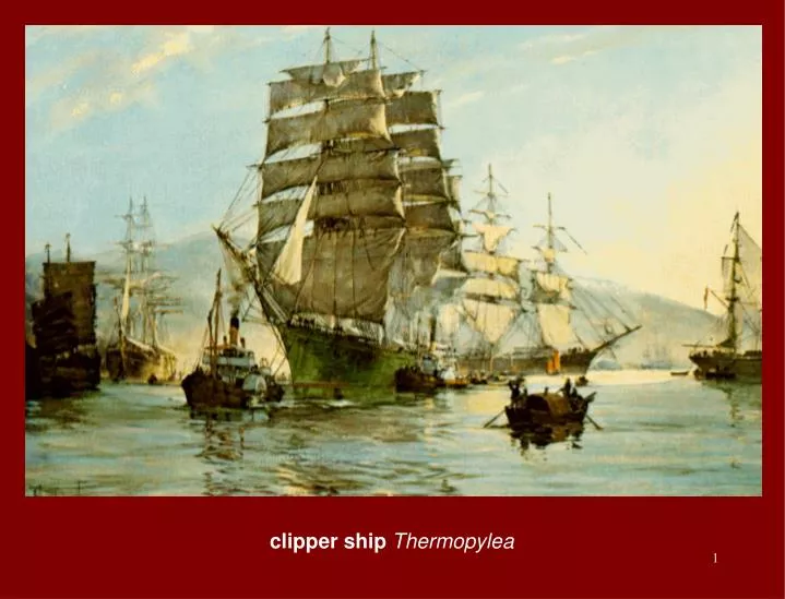
clipper ship Thermopylea. ocean circulation basic current models.

E N D
Meant for several classmates that have asked for more information about the scope of this portion of the course, here is an overview of the ocean physics involved, in graphical format : the graph above has all the fluid motion responses caused by physical forces operating on the ocean. It is not an ordinary linear x-y graph. It is three-dimensional in length [L], time [P], and has relative energy on the third, vertical axis. The horizontal plane is logarithmic [base 10] in both directions and has the virtue of covering an enormous range of distance, in centimeters, and range of time, in seconds. Note that the longest distance one can measure, point-to-point, is bounded by the size of the Earth. The time scale runs from less than a minute to thousands of years. There is an enormous amount of energy involved in ice ages and the changes they invoke in the environment. Something we do not have much chance to normally observe, but didn’t someone say our polar regions are melting ? We see and know about astronomical tides, the double, narrow strips at 12 and 24 hours. Our present ocean circulation studies are in the geostrophic region of the graph, relatively inconspicuous, but very important for the Earth. The spatial scales of the features therein are hundreds to thousands kilometers and the temporal scales from days to years. We are going to focus on the very long-term average features in these ranges; for example, we will examine the vastly different characters of the central subtropical and subpolar gyres.
The surface movement of the world ocean includes five major permanent gyres, North Atlantic, North Pacific, South Atlantic, South Pacific, and the Antarctic Circumpolar regimes. Another, the Indian Ocean gyre, is permanent as well, as is its yearly reversal associated with Monsoon winds. The correlations with atmo-spheric processes are clear and show the extent of interactions and ongoing links within an air-sea system on Earth.
There are reasonable positive correlations to be seen between the major features in the surface flow regimes and surface wind systems. We will look at those shortly. But a clue about what lays ahead lies in answer to this question : What are the sources of the particular spatial physical and chemical and biological distributions evident in the world ocean ? Oceanographic research over the last 100 + years has provided a base of hydrographic, current meter, drifter and satellite data that support analyses establishing the average, long-term flow conditions that prevail. Such an average procedure smooths out short-term fluctuations and tells oceanographers what can usually be expected at any time over the world’s ocean. The density of the data is much greater in some geographic locations and some of the flow patterns shown in the last slide could benefit with additional observations in some regions. Never-the-less, we believe that we have information on what is where in most regions and also understand what fluctuations can and will occur over time spans <100 years. As an example, In ocean current studies we tend to speak of short-term fluctuations of less than a year as related to flow instabilities and turbulence. Such features are not present in the distribution you have just examined, they have been averaged away. Even so, one important use of a physical distribution like those is to find relationships that it bear on biological, chemical and geological distributions. Gaining knowledge of those relationships helps us understand how the ocean system has worked recently and possibly over eons in the past. Our goal will be comparison of average distributions of oceanic biological, chemical and physical features so you can learn how they jointly influence one another and how they maintain the system of which they are part. We will begin by studying the important long-term features of circulation in terms of the forces that maintain them :
Coriolis : the influence of Earth’s rotation Recall our discussion of the perception of motion. Observations of motion require some index against which to measure, that is, a coordinate system of some type with which we assess an object’s trajectory. The models we use to study the ocean and understand its physics are expressed and measured in a rotating spherical geographic coordinate framework in which position is given in latitude and longitude. The inclusion of the effect of the Earth’s rotation is necesary in models that describe and predict oceanic motion because we describe and predict on a rotating coordinate system. In class and with the atmosphere power point we saw how that bit of retrograde Mars motion came about. We then asked Isaac Newton to give us his analysis of the segment of Mar’s trajectory without identifying the object. The description of the trajectory was made with his First Law, that is, with Galileo’s Law of Inertia, and concluded this : the evident deviation from a straight line motion at constant speed means some force is at work on an object. However, we know that the deviation is there because of the relative motion of Mars and the earth-bound coordinate system. Coriolis is included as a real force in ourmodels of the ocean even though it can deliver neither a pull or push in our world. Without the ability to push or pull, the Coriolis Force cannot do work, and that is the actual measure of “real” for a force. But if Coriolis is not treated as a force in our ocean models, then the models will fail in both descriptions or predictions of motion in the rotating coordinate system we are bound to use. Coriolis force is an important force in all our ocean models. Count this as our first necessary force to consider.
wind on the water Compare surface winds and currents. Granted the wind pattern is for January, yielding a positive monsoon correlation in the Indian ocean with a climatic mean current pattern. Yet, the comparison is positive over all the other ocean basins as well. We can expect that the horizontal component of the force of wind on water, known as the wind stress, will play an important role in our 251 models of ocean circulation. What may be unexpected for you is the fact that wind plays a dynamic and im-portant role in the ocean’s vertical motions, as well. Wind stress is our second important force in circulation. surface winds surface currents
gravity and its pressure effect in the water Since gravity on earth gives objects their weight, a column of water extending in the ocean from its surface to some horizontal surface at depth will, by its weight, exert pressure on that surface. Now pressure is a different sort of force : it has a certain strength (magnitude) in, say, pounds per square inch, but it acts in all directions at once. Think of blowing up a balloon and sticking a pin in it. Pressure forces air out of the pinhole in a direction perpendicular to the balloon’s surface at the pinhole; no matter where you make the pinhole. Pressure acts in all directions at once ! Suppose ocean water has the same density everywhere. Now consider columns of water at two different locations, and have one column of different height. The weight of each column is different at our chosen horizontal surface at depth and therefore the pressure has two different values at two different positions on the same horizontal surface. Without exception, the water will want to move along the horizontal surface from the position under the column of high pressure to the position under the column of low pressure. So, in a sense we have converted the vertical force of gravity into a horizontal force that is the equivalent to the difference in pressure between the locations of the columns; we call that force a pressure difference force, or more commonly put : a pressure gradient force. This pressuregradient is the third major force influencing the ocean’s flow for us 251ers to consider. Friction is another useful influence to consider. We will have occasion to invoke friction in our explanations of the interactions between wind and water, between different waters and between water and land. But before we proceed, remember that there are different water masses of different temperature and salinity to be found from surface to depth within the ocean. And therefore we will find different density waters in any water column of a real ocean. So we should understand that part of a pressure gradient force in the ocean can be brought about by different density waters within a given column of water.
Ekman Model Approach The issue herein is momentum that is transferred by a frictional force [a stress] across a horizontal interface, from one fluid layer to another of dissimilar density. The initial layers are air and water and the interface is the sea surface. Other pairs lie below in layers and are considered in sequence with increasing depth. A physical constraint on the mathematical solution dictates that stronger winds must cause deeper penetration of the current response into the layered ocean. The effect of including Coriolis, that is accounting for rotation of the model’s coordinate system, produces a model flow directed to the right of the wind stress direction in the northern hemisphere, that is, to the right of the force balance. This flow is the response of the lower layer to the stress applied by the upper layer and marks the downward transfer of momentum by frictional interaction between the layers. This effect continues with depth, layer-to-layer, as the model layer currents swing to the right and diminish in strength. We refer to this as the Ekman spiral.
Ekman model results We use this model and its result as a start point to discuss circulation. First of all, when at depth the flow is in the direction opposite to the surface flow direction, we can define an interval known as the Ekman depth. The average flow over this depth interval is an important result for the description of circulation in the open ocean as well as on continental shelves.
Here is a question for you : if the model forces are in balance, how can there be motion ? One can have motion and a force balance. Newton’s laws are specific, no acceleration along the axis of a force balance because there is no net force. The F in [F = ma] sums to zero and since the mass has a real value, acceleration must be zero, ie, no velocity change. Motion could be allowed at constant speed along the force axis. If the physical situation warrants it. Nothing said about motion perpendicular to the balance axis either. So one may remain consistent with Newton’s laws of motion when model motion is perpendicular to the force balance.When we average over the Ekman Depth, we find this latter circumstance and oceanographers refer to that moving mass of water [light blue arrow above] as net transport. It is perpendicular to the direction of the wind [and the balance] and Newton is satisfied. Note 1 : the stronger the wind the deeper the Ekman Depth and the greater the net transport. Note 2 : in the southern hemisphere, the spiral and net transport are to the left of the axis of balance and the direction of the wind. Next question : does this model result relate to actual features and processes in the ocean ?
Observations have shown a clear correlation between the horizontal motion of major atmospheric wind systems and movement of underlying oceanic gyres. We can apply the Ekman model to attempt explanations of vertical motions In the same gyres. As an example : Prototypical, northern hemisphere sub-tropical gyres centered at 30 degrees are spun clockwise in direct response to wind torque applied by the NortheastTrade and Westerly winds. In addition, Ekman model results predict that these winds maintain a central mound of water within a gyre through the presence of inward Ekman net transport toward its center. [Note the orientation of the broad blue-green arrows on the left.] Sub-tropical gyres are called convergent for this reason. Does such an elevation exist ? If so, how does it relate to the known flow pattern ? For decades, hydrographic observations and their analyses with the Geostrophic model have yielded current estimates from pressure gradients that implied mounds of water present within subtropical gyres. And the Ekman model provided an explanation of a mound’s presence. Recent satellite observations have confirmed this mound as an actual topographic feature.
upwelling along coastlines … for instance, along the US west coast, most of the year,over the continental shelf, winds blow with a strong southward component, generating offshore flow and upwelling near the coast …. the upwelled water is cold and nutrient rich …. the nutrients support the growth of phytoplankton and, through the food chain support rich fisheries …. The cold up-welled water also sells a lot of wet suits to the surfers …..
The effect of the Trade and Westerly Winds in an Ekman model would be to maintain a more-or-less symmetric water elevation centered approx-imately along 30 degrees north or south latitude. For the northern hemisphere :
Geostrophic Model Approach Differences in water pressure [pressure gradient] along a level surface at depth in the ocean constitute a force that can induce motion along that surface from high to low pressure locations. The water pressure on any level surface can be approximated by the weight [W] of the water column above its depth; W = mg. This is Newton’s second law [ F = ma : mg = W ] wherein the g is the acceleration of gravity. How could one estimate the mass of the water m above the level surface ? Take a CTD hydrocast with the ship, calculate the density of the seawater as it varies along the vertical on the cast, and find the required mass from density. Repeat at another location on the ocean and take the difference in pressure to find the pressure gradient force. On the level surface between station loca-tions, water is urged to move from high to low pressure. For the steady-state geostrophic current model, the pressure gradient force is balanced by the Coriolis force and the movement of the water is taken to be perpendicular to a line joining the station locations. In the northern hemisphere, the direction of geostrophic model flow is to the right looking down the pressure gradient.
To estimate the pressure gradient for current strength calculations using the Geostrophic model’s results, oceanographers require at least two hydrographic stations to assess density and hence pressure at some chosen depth under the two water columns. To illustrate the process, we take one station at the center of the elevation [B] and one at the edge [A]. The station separation for a whole gyre like this would require a variable interval; perhaps twenty kilometers in high speed regions like the Gulf Stream, 50 kilometers elsewhere. The interval or sequence of intervals normally depends on the observational intent of the field program .
schematic of a station sequence useful for our ideal symmetric water elevation
1. The Nansen bottle was used extensively by ocean-ographer until the 1970s. The first cruise using all electronic sensing for salin-ity by Woods Hole Ocean-ographic Institution was in 1969. The Nansen bottle continued in use and was reliable but provided data eventually insufficient for complex research intents. Rosette Sampler Niskin bottles Nansen bottle tripping 2. Today’s CTD [conductivity, temperature, depth] relies on electronic instrumentation and telemetry to deliver spatially dense data sets. It is a high initial cost and high main-tenance instrument. CTD
The Geostrophic model applied to a northern hemisphere subtropical gyre. Note the blue current vector’s direction, to the right of the balance looking down the pressue gradient What then are we to expect for a northern hemisphere subpolar gyre?
Polar Easterlies Westerlies A subpolar gyre is a converse situation relative to a subtropical gyre, in which the polar easterly and westerly winds act to produce a sea surface that is lower than usual and spin waters in a counter-clockwise direction. Horizontal, divergent surface motion away from the gyre center and a directly associated vertical upwelling is indicated by the Ekman transport model. Subpolar gyres are known as divergent gyres in view of the outward radial motion. Mound or depression, are they real or model artifacts ?
An overview of the world ocean was obtained by a radar system flown on the SEASAT NASA satellite. By appropriate selection of radar microwave characteristics, an analysis of the radar return signals provided accurate observations at a spatial resolution that yields useful topography of the sea surface. Satellite passes revealed topography along the satellite subtrack, the projection of the orbital path onto the Earth’s surface. The red line on the above chart is a portion of a subtrack that extends over shallow continental shelf waters on the left to Sargasso Sea waters on the right. The red line on the graph traces the sea surface topography over the extent of the partial subtrack. On the far right, the steep gradient of approximately 140 cm per 100 kilometers locates the north wall of the Gulf Stream, here a boundary between colder and fresher Mid-Atlantic Waters and Sargasso Sea Waters. Then there is a mound, albeit one that is shifted westward with respect to the central portion of the subtropical gyre, the Trade and Westerly wind systems, and the more-or-less symmetric water feature we expected on the basis of Ekman Theory. Next question : Why is there westward distortion of the elevated mound ?
Be sure you can identify the actual currents around the gyre in the Atlantic basin and the Pacific basin. What’s that red line ? The white contours are a schematic of the atmospheric circulation over the North Atlantic Ocean and the blue contours indicate the corresponding wind-driven ocean circulation. This illustration is based on many years of observation and stands for the long-term-average relationship between atm and ocn in this region. Count on it. About 80% of the time. Why are the blue contours crowded against the North American continent’s east coast ? Because of Galileo. And his law of inertia, that Newton cribbed. The law of inertia states : leave me alone will you, I’m doing my thing here. Translated, as the Earth rotates from west to east, the ocean, free on the planet’s surface, is crowded much by the NA continent and the ocean just hangs there, more and more against the shore and tends to pile up, go look at the red line, slide 20.
Note that, in reality, the broad and shallow Canary Current must carry approximately the same volume of cooler water southward as the narrow deep and warmer flow of the Gulf Stream carries northward. A model would insist on this as well as have a current similar to the North Equatorial Current flowing westward to the south that matched the volume of the branch of the North Atlantic Current bringing water eastward in the north. In a model this conservation of mass is regarded as maintaining continuity of the flow pattern.
Remember, these patterns are long-term means we expect to be there . The means underlie smaller scale spatial and temporal fluctuations associated with turbulence and mixing in the ocean. How does the variability associated with the Gulf Stream appear in our observations ?
Our ocean current studies have considered steady-state physical situations because time dependent models are beyond our mathematical skills in OCNG 251. The temporal changes in ocean currents [and atmospheric winds] are extremely important as they achieve the transport and mixing of anomalous quantities that could disturb and alter the environmental conditions supporting climate and life in the ocean and therefore our world. At that, the balance models we have will, in the open ocean away from land boundaries, successfully portray current characteristics and provide flow estimates that are sufficient for a fundamental understanding of the oceanic system. For a moment, lets take a look at examples of the time-dependent portion of the ocean’s movement :
Fluctuations In a major current like the Gulf stream are related in a time-lagged sense to fluctuations in the atmosphere. The variability in current speed and direction induced by changes in the driving force can, if large enough, produce relatively small instabilities in the flow of a major current; these instabilities can grow and develop unique eddies that spin away within the parent current’s environment. This is the mixing process mentioned in slide 23. The repeated satellite passes along the track shown above have captured, from west to east, the shifted mound of water, the Gulf Stream’s north wall, and a “dimple” on the surface of the Sargasso Sea which marks the position of a cold core eddy or ring drifting across the subtrack line at a latitude of 34 - 35 degrees north latitude? What was the origin of this feature and what is its role in circulation ?
In view of the large current data base gathered for over a century or more, we place considerable confidence in regarding the flow patterns shown in the previous slide as one aspect of ocean climate, the mean motions that one can expect out there. In terms of the western North Atlantic, This infrared satellite sensing of the surface temperature appears much different than smooth mean currents. The Gulf Stream northeast of Cape Hatteras meanders extensively and there are the telltale indications of circular features, north and south of the Stream, that are turbulence in the form of mesoscale eddies generated from current instabilities. The eddies, known as Gulf Stream rings, break off from the parent flow when a meander pinches off at its neck. If we see our way clear to identify the patterns on the last slide as climate, then rings are local weather and storms. About ring structure : trapped within each ring are waters that come from the other side of the Stream that are surrounded by a Gulf Stream remnant. This is the initial form of the large scale mixing process that distributes anomalies of temperature and salinity in the ocean. The rings are as large as 200 km in diameter and last as long as nine months as they spin and mix themselves into their background. A schematic sequence of cold core [blue] ring generation, to the south of the Stream, is shown below :
Big whirls have little whirls which feed on their velocity. Little whirls have lesser whirls and so on to viscosity. This satellite infrared image illustrates the generation of a warm core [yellow] ring that was about to separate from the Gulf Stream [red] and enter the Mid-Atlantic Bight [blue] off New York City [upper left] in the Spring of 1982. The surface temperature range is more than twenty centigrade degrees and the smooth variation from blue through green to yellow indicates the ongoing mixing that is smoothing out this positive temperature anomaly. The physical fluid dynamic interactions between ring and background are suggested in the above ditty, most recently quoted by LF Richardson. It gives a prescription for the eventual dissolution of the eddy by distributing its energy into its environment. Look for the lesser whirls around the ring that are part of the turbulence accomplishing this important physical process.