Download
1 / 13
140 likes | 433 Views
MESB 374 System Modeling and Analysis Inverse Laplace Transform and I/O Model. Inverse Laplace Transform. Basic steps Partial fraction expansion (PFE) Residue command in Matlab Input-output model by using Laplace transform. Inverse Laplace Transform.

E N D
MESB 374 System Modeling and AnalysisInverseLaplace Transform and I/O Model
Inverse Laplace Transform • Basic steps • Partial fraction expansion (PFE) • Residue command in Matlab • Input-output model by using Laplace transform
Inverse Laplace Transform Given an s-domain function F(s), the inverse Laplace transform is used to obtain the corresponding time domain function f (t). Procedure: • Write F(s) as a rational function of s. • Use long division to write F(s) as the sum of a strictly proper rational function and a quotient part. • Use Partial-Fraction Expansion (PFE) to break up the strictly proper rational function as a series of components, whose inverse Laplace transforms are known. • Apply inverse Laplace transform to individual components.
Partial Fraction Expansion • Case I: Distinct Characteristic Roots • Residual Formula • Proof
Partial Fraction Expansion • Case II: Repeated Roots • Residual Formula • Proof
Partial Fraction Expansion • Case III: General Case • Residual Formula
Partial Fraction Expansion • Case IV: Order of the Numerator C(s) = Order of the denominator D(s) : n = m
Partial Fraction Expansion • Case V: Complex Roots
[A, P, K] = residue (num, den) num:vector of coefficients of the numerator; Den:vector of coefficients of the denominator; A:vector of the coefficients in PFE, i.e., P: vector of the roots, i.e., K: constant term. Residue Command in MATLAB
Residue Command in MATLAB (Example) Ex: Given Find: inverse Laplace transform MATLAB command: >> [A, P, K] = residue ( [1, 0, 0, 2] , [1, 2, 1, 0] ) will return the following values: A = [ -4, -1, 2]T , P = [ -1, -1, 0] , K = 1 which means that
Obtaining I/O Model Using LT(Laplace Transformation Method) • Use LT to transform all time-domain differential equations into s-domain algebraic equations assuming zero ICs • Solve for output in terms of inputs in s-domain • Write down the I/O model based on solution in s-domain
Example – Car Suspension System x p • Step 1: LT of differential equations assuming zero ICs • Step 2: Solve for output using algebraic elimination method • # of unknown variables = # equations ? 2. Eliminate intermediate variables one by one. To eliminate one intermediate variable, solve for the variable from one of the equations and substitute it into ALL the rest of equations; make sure that the variable is completely eliminated from the remaining equations
Example (Cont.) from first equation Substitute it into the second equation • Step 3: write down I/O model