Download
1 / 43
430 likes | 574 Views
NHSC/PACS Web Tutorials Running the PACS Spectrometer pipeline for CHOP/NOD Mode PACS-301 Pipeline Level 0 to 1 processing. Prepared by Dario Fadda Updated by Babar Ali, February 2013 Updated by Steve Lord, Oct 2013. Introduction

E N D
NHSC/PACS Web Tutorials Running the PACS Spectrometer pipeline for CHOP/NOD Mode PACS-301 Pipeline Level 0 to 1 processing Prepared by Dario Fadda Updated by Babar Ali, February 2013 Updated by Steve Lord, Oct 2013
Introduction This tutorial will guide you through the interactive spectrometer pipeline from loading raw data into HIPE to obtain calibrated data with astrometry in the case of chop/nod mode. Pre-requisites The following tutorials should be read before this one: • PACS-101: How to use these tutorials. • PACS-102: Accessing and storing data from the Herschel Science Archive • PACS-103: Loading scripts • Sequel: PACS-302 – Level 1-2 processing
Overview Step 1 Check HIPE version and your local memory Step 2 Set up script for the particular Obs ID Step 3 Run the 0 → 0.5 pipeline Step 4 Run the 0.5 → 1 pipeline
Step 1 Check HIPE version and memory allocation The version used for the tutorial is 11.0 build 2938
Select “about” from the drop down Help menu A pop-up window with the HIPE version appears
To allocate memory, select preferences under edit, then ... N.b.:, Memory used and available
…click on “Startup & Shutdown” and change the amount of memory The allocated memory should be a bit smaller than the total RAM of your computer. (e.g. 7.5 out of 8.0 Gbytes) You must exit and restart HIPE to obtain the new amount of memory.
Step 2 Setup Load pipeline script; load observation; check your data; and select the camera
Loading the script The “linescan” script used in this tutorial corresponds to the script available directly from the distribution.
Loading the observation Once the script is loaded, one simply steps through the lines to execute it. But first modify it for OBSID of the observation desired. In the case of this tutorial, the observation was already saved into a pool in the user’s local ~/.hcss/lstore directory (created when first installing HIPE). So one modifies the obsid in the script and clicks through using the green arrow…. Hit the green arrow to step through the entire script Modify this line. Here we set obsid to 1342186799.
Loading the observation If the data is not stored as a local pool, you want to tell the script to acquire the data from HSA. In this case edit the line to useHsa=1
Loading the observation Next step, we load the observational context ( a structure containing all the observational data, information about them and calibration data). Click through this line using the green arrow.
Observation Selection For this data set, we will concern ourselves with the line observed in the PACS blue channel. Click through (using the green arrow) the remaining lines, choosing your preferences as described in the comments until you get to the channel section.
Setting the camera We select camera = 'blue' After selecting the camera, we can check what camera we selected by simply printing: “print camera”
Setting the calibration tree Finally, we set the calibration tree. This reads the time stamp of our obs and applies the calibration from the appropriate calibration tree. The Cal trees can be accessed and updated from Preferences > Data Access > Pacs Calibration. • print obs.meta[“calVersion”] shows the calibration used in current observation.
Step 3 Run the 0 → 0.5 pipeline Basic calibration (pointing, wavelength calibration, slicing)
Level 0 → 0.5 Wavelength Calibration PACS data, House Keeping Raw data Pointing Data flagging Permanently Bad pixels When grating or chopper moving Saturated data Open and dummy channels DNs to Volts/s conversion Assign observing block labels (e. g. Nod positions, grating scan direction, calibration block, scan mode) Assign RA/Dec to pixels Level 0.5 Sliced Frames 16 x 25 x ramps Grating to wavelength
Check: level 0 From now on, we will step through the script line by line using the green arrow on the menu bar. The first step consists in extracting the 0-level products from the observation context. 2nd line Calibration block 1st line, 3 repeats The plot appears after: ‘p0 = slicedSummaryPlot(slicedFrames,signal=1)’ In our case, after the calibration block, we can identify two different lines observed 3 times in the two nod positions.
Continue … With remaining Level 0 to 0.5 processing steps as outlined in slide 17. Step through with the green arrow.
Check: footprint Nod A Nod B
Continue … With remaining Level 0 to 0.5 processing steps as outlined in slide 17. Step through with the green arrow.
Check: after slicedSummaryPlot(slicedFrames…) Nod B Nod A Cal Block There are two lines (two wavelengths in red). Grating scans are numbered positive if upscans and negative if downscans.
Check: slcedSummary(slicedFrames) The slicing of the data is performed according to rules made explicit in the pipeline. In our example, two lines are observed in two nodding positions. So, we expect 4 slices plus an initial slice containing the calibration block.
Check: after slicing 5 slices ! Line 1 – B & A nodes Line 2 – B & A nodes
Check: after slicing Line 1: OI 63 Line 2: NIII 57 Cal Block There are four slices (calibration, nod A and B for the 1st line, nod A and B for the 2nd line).
Continue … With remaining Level 0 to 0.5 processing steps as outlined in slide 17. Step through with the green arrow.
Step 4 Run the 0.5 → 1 pipeline Glitch detection, chop differentiation, RSRF, flat
Glitch detection Apply RSRF Apply nominal response Subtract On and Off Chop Frames to Cubes Second level deglitching & rebinning Spectral Flat Fielding Level 0.5 → 1 Level 0.5 Level 1
Diagnostics With verbose=1 (earlier in the script) several diagnostic plots and print out (watch your console) will appear after these lines …
Check: Glitch detection You can check manually the points flagged as glitches or masked for other reasons using the maskviewer Select a pixel by clicking on it Do first Select a mask Select a frame Current frame Masked glitch ON signal OFF signal
More masks It is possible to explore other masks Select unclean chop In this case, it is clear why there is a second group of points for the ON and OFF positions. These corresponds to signals obtained when the chopper was not yet in the correct position.
Look for this new tab in your editor window. Adjust screen to match this view. A further inspection of your data is now possible using the Spectrum Explorer. Several options are available such as selection of pixels and different masks for the first slice.
Continue … With remaining Level 0.5 to 1.0 processing steps as outlined in slide 28. Step through with the green arrow.
Chop differentiation Verbose=1, shows After chop differentiation, the calibration block is excluded from the data
Chop differentiation Verbose=1 shows The data are only on the ON position (OFF being subtracted)
Continue … With remaining Level 0.5 to 1.0 processing steps as outlined in slide 28. Step through with the green arrow.
Check: RSRF and response After pb4ff = plotPixels(slicedCubes.get(…….. After applying RSRF and response corrections we have a first look at the spectrum
Continue … With remaining Level 0.5 to 1.0 processing steps as outlined in slide 28. Step through with the green arrow.
Check: Spectral FlatField As a default, the code will search for lines in all the pixels and then mask them before computing the spectral flat field. It is possible to give directly the list of lines to be masked via the parameter lineList = [63.227], for instance.
Continue … With remaining Level 0.5 to 1.0 processing steps as outlined in slide 28. Step through with the green arrow.
Check: Spectral FlatField At this point, the frames are converted in calibrated cubes and we have reached level 1 !