Download
1 / 23
230 likes | 397 Views
Approximate Convex Decomposition of Polygons. Jyh-Ming Lien Nancy M. Amato {neilien, amato}@cs.tamu.edu Parasol Lab.,Department of Computer Science Texas A&M University ACM Symposium on Computational Geometry 2004[32]. 多边形的凸剖分: 利用对角线 剖分为一组凸多边形. 凸剖分的意义: 凸物体更易于操作 很多算法对于凸的物体更加有效

E N D
Approximate Convex Decomposition of Polygons Jyh-Ming Lien Nancy M. Amato {neilien, amato}@cs.tamu.edu Parasol Lab.,Department of Computer Science Texas A&M University ACM Symposium on Computational Geometry 2004[32]
多边形的凸剖分: 利用对角线 剖分为一组凸多边形
凸剖分的意义: 凸物体更易于操作 很多算法对于凸的物体更加有效 应用领域: 计算机图形学 模型识别 Minkoski sum computation Motion planning Origami folding
多边形凸剖分局限性: 计算量大,耗时 剖分结果不理想,分块数太多且不易控制 多边形“近似”凸剖分: 剖分结果:“近似”凸多边形 类似的应用价值 剖分块数显著减小,计算更加有效 改善一些实际应用的结果
已有工作可归类为: 输入多边形:简单多边形,带洞或不带洞 剖分方法:允许或不允许有Steiner点 输出的剖分结果:最小剖分数目或最短周长 带洞:无论哪种最优条件,都是NP-难 不带洞:最小剖分数目:不允许Steiner点时 允许时 最短周长:不允许Steiner点时 允许时 :尚未有最优解 无最优要求时: 本文结果:
本文的工作: 对任意的简单多边形,带洞或不带洞 提供一个机制,关注于关键特征进行处理 给出不同近似水平上的近似凸剖分系列表示
一些定义: concave(P): notch-----凹顶点 bridge------- pocket------
算法 Approx_CD(P, ) 输入:多边形P,凹度容差 输出: c=concave (P) if c.value< return P else { }=Resolve(P, c.witness). for i=1,2 do Approx_CD( , ).
Resolve (P, r ): 在凹顶点r处添加对角线使之不再凹。 r在外边界上时, 取r处的角平分线; r在洞的边界上时, 取外边界上离r最近的顶点, 连线
度量凹度: 面积比 曲率
度量外边界的凹度: SL_Concavity: 直线距离 经剖分后凹度可能会增加 不能很好反映凹度
SL_Concavity: 对于由pocket 和bridge 构成的简单多边形 , 对 上每个顶点x都找一条到边 的完全在 中的最 短路径 ,它的长度即为x的凹度。
把多边形 分为三部分 、 、 。 对于 和 ,最短路径可在 和 处的visibility tree中找到, 对于 ,可把其顶点分为两类 、 。 中顶点的最短路径必然过 中的顶点。
算法SP_Concavity( , ) 把多边形 分为三部分 、 、 。 分别以 和 为根对 中顶点构造visibility tree 和 。 ,在 ( )中计算最短路径 。 由 和 计算 中的一个有序点集 。 for ,do for i<k<j do 。 return {x , c} ,其中x是具有到 最远距离c的 中顶点。
算法复杂度O (n)。 多边形的凹度随剖分单调递减。
Hybrid Concavity( H-Concavity) SL_concavity: 简单,计算容易 SP_concavity: 更加有效,且随剖分单调递减 考虑一个混合模式,兼具它们的优点。
算法H1-Concavity( , ) if , s.t. then return SL-concavity and its witness. else return SP-concavity and its witness. 算法H2-concavity( , ) 1. SL-concavity and its witness {x , c}. 2. if then return {x , c}. 3. if , s.t. then return {x , c}. 4. return SP-concavity and its witness.
洞的凹度 精确求解p、cw(p)的复杂度 近似求解:中轴线法( medial axis) 主轴线法(principal axis)
中轴线法对应于SP_concavity 主轴线法对应于SL_concavity 对于每个洞 ,找到一对 和 ,以及离 最近的顶点x, 连接 。
总体算法的复杂度: 设多边形P具有n个顶点,r个凹顶点,k个洞,则P的近似 分解的时间为O(nr). 证: 求凸包,bridge, pocket都是O(n). 度量凹度, 求凹度最大点是O(n)(SL,SP,H1,H2). resolve子程序也是O(n),所以每轮循环是O(n). 由于每剖分一次,最多产生三个新顶点,设最终分解为m块, 则循环次数为m-1,总的时间为:
有洞时,度量凹度需要O(n)时间,添加对角线需要O(n)时间,有洞时,度量凹度需要O(n)时间,添加对角线需要O(n)时间, 每次处理一个洞最多产生3个新顶点,所以类似于前面,它需要 时间。 总的剖分时间为 由于m<=r+1, k<r,r<n,