An Overview of the AMMA Multi-Model Intercomparison project

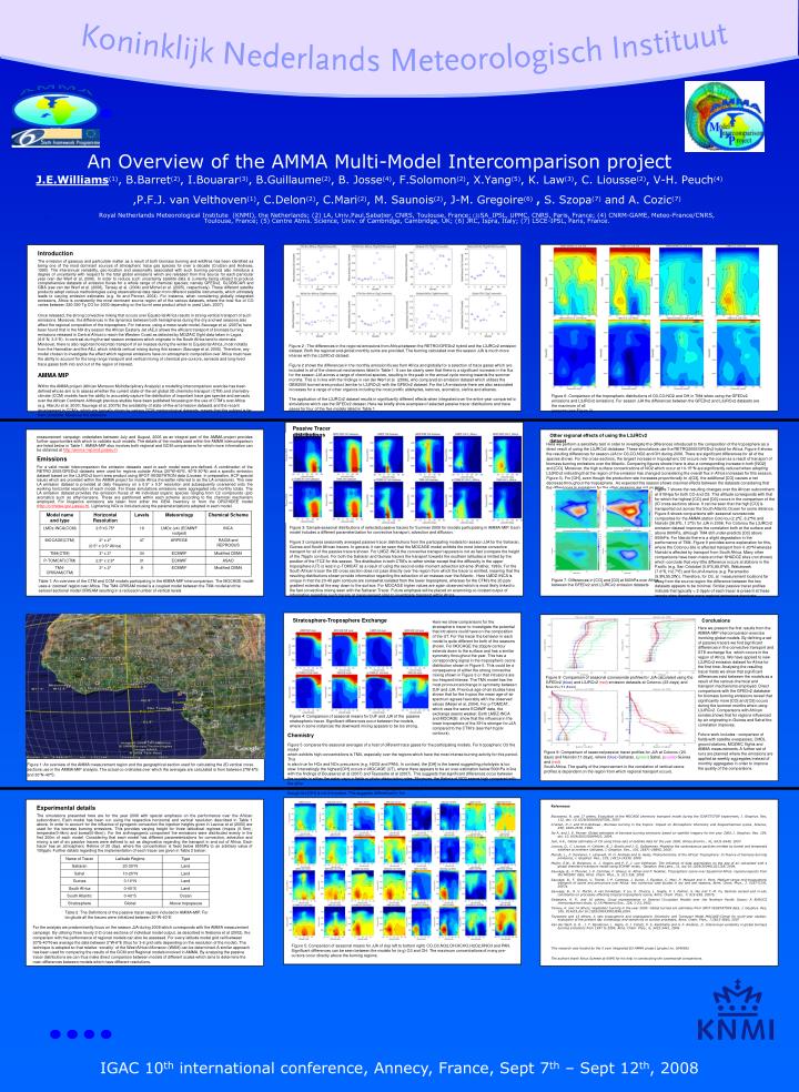
1. An Overview of the AMMA Multi-Model Intercomparison project J.E.Williams(1), B.Barret(2), I.Bouarar(3), B.Guillaume(2), B. Josse(4), F.Solomon(2), X.Yang(5), K. Law(3), C. Liousse(2), V-H. Peuch(4) ,P.F.J. van Velthoven(1),C.Delon(2), C.Mari(2), M. Saunois(2), J-M. Gregoire(6) , S. Szopa(7)and A. Cozic(7) Royal Netherlands Meteorological Institute (KNMI), the Netherlands; (2) LA, Univ.Paul.Sabatier, CNRS, Toulouse, France; (3)SA_IPSL, UPMC, CNRS, Paris, France; (4) CNRM-GAME, Meteo-France/CNRS, Toulouse, France; (5) Centre Atms. Science, Univ. of Cambridge, Cambridge, UK; (6) JRC, Ispra, Italy; (7) LSCE-IPSL, Paris, France. Introduction The emission of gaseous and particulate matter as a result of both biomass burning and wildfires has been identified as being one of the most dominant sources of atmospheric trace gas species for over a decade (Crutzen and Andreae, 1990). The interannual variability, geo-location and seasonality associated with such burning periods also introduce a degree of uncertainty with respect to the total global emissions which are released from this source for each particular year (van der Werf et al, 2006). In order to reduce such uncertainty satellite data is currently being utilized to produce comprehensive datasets of emission fluxes for a whole range of chemical species; namely GFEDv2, GLOBSCARand GBA (see van der Werf et al. (2006), Tansey et al. (2004) and Michel et al. (2005), respectively). These different satellite products adopt various methodologies using observational data taken from different satellite instruments, which ultimately leads to varying emission estimates (e.g. Ito and Penner, 2004). For instance, when considering globally integrated emissions, Africa is consistently the most dominant source region all of the various datasets, where the total flux of CO varies between 320-390 Tg CO for 2000 depending on the burnt area product which is used (Jain, 2007). Once released, the strong convective mixing that occurs over Equatorial Africa results in strong vertical transport of such emissions. Moreover, the differences in the dynamics between both hemispheres during the dry and wet seasons also affect the regional composition of the troposphere. For instance, using a meso-scale model, Sauvage et al. (2007a) have been found that in the NH dry season the African Easterly Jet (AEJ) allows the efficient transport of biomass burning emissions released in Central Africa to reach the Western Coast as detected by MOZAIC flight data taken in Lagos (6.6N, 3.3E). In contrast during the wet season emissions which originate in the South Africa tend to dominate. Moreover, there is also regional (horizontal) transport of air masses during the winter to Equatorial Africa, most notably from the Harmattan and the AEJ, which inhibits vertical mixing during this season (Sauvage et al, 2005). Therefore, any model chosen to investigate the effect which regional emissions have on atmospheric composition over Africa must have the ability to account for the long-range transport and vertical mixing of chemical pre-cursors, aerosols and long-lived trace gases both into and out of the region of interest. AMMA MIP Within the AMMA project (African Monsoon Multidisciplinary Analysis) a modelling intercomparison exercise has been defined whose aim is to assess whether the current state-of-the-art global 3D chemistry-transport (CTM) and chemistry-climate (CCM) models have the ability to accurately capture the distribution of important trace gas species and aerosols over the African Continent. Although previous studies have been published focussing on the use of CTM’s over Africa (e.g. Marufu et al, 2000; Sauvage et al, 2007b) the availability of state-of-the-art emission datasets and the recent development in CCM’s, which are typically driven by various GCM meteorological datasets, means that this subject is far from complete. Moreover the intensive Figure 2 : The differences in the regional emissions from Africa between the RETRO/GFEDv2 hybrid and the L3JRCv2 emission dataset. Both the regional and global monthly sums are provided. The burning calculated over the season JJA is much more intense with the L3JRCv2 dataset. Figure 2 shows the differences in the monthly emission fluxes from Africa and globally for a selection of trace gases which are included in all of the chemical mechanisms listed in Table 1. It can be clearly seen that there is a significant increase in the flux for the season JJA across a range of chemical species, resulting in the peak in the annual cycle moving towards the summer months. This is in line with the findings in van der Werf et al. (2006), who compared an emission dataset which utilises the GBA2000 burned area product (similar to L3JRCv2) with the GFEDv2 dataset. For the LA emissions there are also associated increases for a range of other organics including the most prolific aldehydes, ketones, aromatics, olefins and alkanes. The application of the L3JRCv2 dataset results in significantly different effects when integrated over the entire year compared to simulations which use the GFEDv2 dataset. Here we briefly show examples of selected passive tracer distributions and trace gases for four of the five models listed in Table 1. Figure 6: Comparison of the tropospheric distributions of O3,CO,NO2 and OH in TM4 when using the GFEDv2 emissions and L3JRCv2 emissions. For season JJA the differences between the GFEDv2 and L3JRCv2 datasets are the maximum of all seasons (see Figure 2). Passive Tracer distributions measurement campaign undertaken between July and August, 2006 as an integral part of the AMMA project provides further opportunities with which to validate such models. The details of the models used within the AMMA intercomparison are listed below in Table 1. AMMA-MIP also involves both regional and GCM comparisons for which more information can be obtained at http://amma-mip.lmd.jussieu.fr. Emissions For a valid model intercomparison the emission datasets used in each model were pre-defined. A combination of the RETRO 2000/GFEDv2 datasets were used for regions outside Africa (20°W-40°E, 40°S-30°N) and a specific emission dataset based on the L3JRCv2 burnt area product using SPOT-VEGETATION data (Liousse, in preparation, ACP special issue) which are provided within the AMMA project for inside Africa (hereafter referred to as the LA emissions). This new LA emission dataset is provided at daily frequency on a 0.5° x 0.5° resolution and subsequently coarsened onto the working horizontal resolution of each model. For these simulations emissions were aggregated into monthly totals. The LA emission dataset provides the emission fluxes of 49 individual organic species ranging from C2 compounds upto aromatics such as ethyl-benzene. These are partitioned within each scheme according to the chemical mechanism employed. For biogenics emissions are taken from either the GEIA inventory or from the ORCHIDEE model (http://orchidee.ipsl.jussieu.fr). Lightening NOx is included using the parameterizations adopted in each model. Other regional effects of using the L3JRCv2 dataset Here we perform a sensitivity test in order to investigate the differences introduced to the composition of the troposphere as a direct result of using the L3JRCv2 database. These simulations use the RETRO2000/GFEDv2 hybrid for Africa. Figure 6 shows the resulting differences for season JJA for O3,CO,NO2 and OH during 2006. There are significant differences for all of the species shown. For the cross-sections, the largest increase in tropospheric O3 occurs over the ocean as a result of transport of biomass burning emissions over the Atlantic. Comparing figures shows there is also a corresponding increase in both [NO2] and [CO]. Moreover, the high surface concentrations of NO2 which occur at 10-15°N are significantly reduced when adopting L3JRCv2 indicating that the region of the emission has changed (considering the overall flux in Africa increases for this season, Figure 3). For [OH], even though the production rate increases proportionally to [O3], the additional [CO] causes a net decrease throughout the troposphere. As expected this season shows maximal effects between the datasets considering that the differences in emissions for the other seasons are not so large. Figure 7 shows the resulting changes over the African subcontinent at 815Hpa for both CO and O3. This altitude corresponds with that for which the highest [CO] and [O3] occurs in the comparison of the 2D cross-sections above. It can be seen that the high [CO] is transported out across the South Atlantic Ocean for some distance. Figure 8 shows comparisons with seasonal ozonesonde composites for the AMMA station Cotonou (2.2°E, 6.2°N) and Nairobi (36.8°E, 1.3°S) for JJA in 2006. For Cotonou the L3JRCv2 emission dataset improves the correlation both at the surface and above 800hPa, although TM4 still under-predicts [O3] above 800hPa. For Nairobi there is a slight degradation in the performance of TM4. Figure 9 provides some explanation for this, where the Cotonou site is affected transport from 0-20°N whereas Nairobi is affected by transport from South Africa. Many other comparisons have been made at other SHADOZ sites (not shown) which conclude that very little difference occurs at stations in the Pacific (e.g. San Cristobel (0.9°S,89.6°W), Watukosek (7.6°S,112.7°E) and South America (e.g. Paramaribo (5.8N,55.2W)). Therefore, for O3, at measurement locations far away from the source region the difference between the two datasets appears to be minimal. Similar passive tracer profiles indicate that typically < 2-3pptv of each tracer is present at these remote sites therefore more regional emissions dominate. Figure 3: Sample seasonal distributions of selected passive tracers for Summer 2006 for models participating in AMMA-MIP. Each model includes a different parameterization for convective transport, advection and diffusion. Figure 3 compares seasonally averaged passive tracer distributions from the participating models for season JJA for the Saharan, Guinea and South African tracers. In general, it can be seen that the MOCAGE model exhibits the most intense convective transport for all of the passive tracers shown. For LMDZ-INCA the convective transport appears is not as fast (compare the height of the 75pptv contour). For both the Saharan and Guinea tracers the transport towards the southern latitudes is limited by the position of the ITCZ for this season. The distribution in both CTM’s is rather similar except that the diffusivity in the upper troposphere (UT) is less in p-TOMCAT as a result of using the second-order moment advection scheme (Prather, 1986). For the South African tracer the 2D cross section does not pass directly over the region from which the tracer is emitted, meaning that the resulting distributions shown provide information regarding the advection of air-masses over the Atlantic . Here LMDZ-INCA is unique in that the 20-40 pptv contours are somewhat isolated from the lower troposphere, whereas for the CTM’s the 20 pptv gradient extends all the way down to the surface. For MOCAGE higher values are again observed which is most likely linked to the fast convective mixing seen with the Saharan Tracer. Future emphasis will be placed on examining co-located output of information regarding such tracers at measurement sites to investigate transport within Africa. Figure 7: Differences in [CO] and [O3] at 800hPa over Africa between the GFEDv2 and L3JRCv2 emission datasets Table 1: An overview of the CTM and CCM models participating in the AMMA-MIP intercomparison. The MOCAGE model uses a ‘zoomed’ region over Africa. The TM4-ORISAM model is a coupled model between the TM4 model and the aerosol sectional model ORISAM resulting in a reduced number of vertical levels Stratosphere-Troposphere Exchange Conclusions Here we show comparisons for the stratospheric tracer to investigate the potential that intrusions could have on the composition of the UT. For this tracer the behavior in each model is quite different for both of the seasons shown. For MOCAGE the 20pptv contour extends down to the surface and has a similar symmetry throughout the year. This has a corresponding signal in the tropospheric ozone distribution shown in Figure 5. This could be a consequence of either the strong convective mixing shown in Figure 3 or that intrusions are too frequent/intense. The TM4 model has the most pronounced change in symmetry between DJF and JJA. Previous age-of-air studies have shown that for the tropics the mean age-of-air spectrum agrees favorably with the observed values (Meijer et al, 2004). For p-TOMCAT, which uses the same ECMWF data, the exchange seems weaker. Both LMDZ-INCA and MOCAGE show that the influence in the lower troposphere of the SH is stronger for JJA compared to the CTM’s (see the10 pptv contours). Here we present the first results from the AMMA-MIP intercomparison exercise involving global models. By defining a set of passive tracers we find significant differences in the convective transport and STE exchange flux which occurs in the region of Africa. We have applied to new L3JRCv2 emission dataset for Africa for the first time. Analysing the resulting tracer fields we show that significant differences exist between the models as a result of the various chemical and transport mechanisms employed. Direct comparisons with the GFEDv2 database for biomass burning emissions reveal that significantly more [CO] and [O3] occurs during the summer months when using L3JRCv2. Comparisons with African sondes shows that for regions influenced by air originating in Guinea and Sahel the correlation improves. Future work includes : comparison of fields with satellite overpasses, CMDL ground stations, MOZAIC flights and AMMA measurements. A further set of runs are planned where the emissions are applied as weekly aggregates instead of monthly aggregates in order to improve the quality of the comparisons. Figure 8: Comparison of seasonal ozonesonde profiles for JJA calculated using the GFEDv2 (blue) and L3JRCv2 (red) emission datasets at Cotonou (23 days) and Nairobi (11 days). . Figure 4: Comparison of seasonal means for DJF and JJA of the passive stratospheric tracer. Significant differences occur between the models, where in some instances the downward mixing appears to be too strong. Chemistry Figure 5 compares the seasonal averages of a host of different trace gases for the participating models. For tropospheric O3 the model which exhibits high concentrations is TM4, especially over the regions which have the most intense burning activity for this period. This is also true for HOx and NOx precursors (e.g. H2O2 and PAN). In contrast, the [OH] is the lowest suggesting photolysis is too slow. Interestingly the highest [OH] occurs in MOCAGE (UT), where there appears to be an over-estimation below 500hPa in line with the findings of Bousserez et al (2007) and Teyssedre et al (2007). This suggests that significant differences occur between the models in either the water vapour fields or photo-dissociation rates. Moreover, the lifetime of NO2 seems high compared with the other models as shown in the [NO2] directly above the burning region. For [CO], p-TOMCAT has the highest concentrations even though the [OH] is not the lowest. This suggests differences in the Figure 9: Comparison of seasonal passive tracer profiles for JJA at Cotonou (23 days) and Nairobi (11 days), where (blue) Saharan, (green) Sahel, (purple) Guinea and (red) South Africa. The quality of the improvement in the correlation of vertical ozone profiles is dependent on the region from which regional transport occurs. Figure 1: An overview of the AMMA measurement region and the geographical section used for calculating the 2D vertical cross-sections use in the AMMA-MIP analysis. The actual co-ordinates over which the averages are calculated is from between 2°W-6°E and 30°N-40°S. • Experimental details • The simulations presented here are for the year 2006 with special emphasis on the performance over the African subcontinent. Each model has been run using the respective horizontal and vertical resolution described in Table 1 above. In order to account for the influence of pyrogenic convection the injection heights given in Lavoue et al (2000) are used for the biomass burning emissions. This provides varying height for three latitudinal regimes (tropics (0-1km), temperate(0-4km) and boreal(0-6km)). For the anthropogenic component the emissions were distributed evenly in the first 300m of each model. Considering that each model has different parameterizations for convection, advection and mixing a set of six passive tracers were defined to act as diagnostics regarding the transport in and out of Africa. Each tracer has an atmospheric lifetime of 20 days, where the concentration is fixed below 850hPa to an arbitrary value of 100pptv. Further details regarding the implementation of each tracer are given in Table 2 below: References Bousserez, N. and 17 others, Evaluation of the MOCAGE chemistry transport model during the ICARTT/ITOP experiment, J. Geophys. Res, 112, doi: 10.1029/2006JD007595, 2007. Crutzen, P..J. and M.O.Andreae., Biomass burning in the tropics: Impact on Atmospheric Chemistry and biogeochemical cycles, Science, 250, 1669-1678, 1990. Ito A. and J. E. Penner, Global estimates of biomass burning emissions based on satellite imagery for the year 2000,J. Geophys. Res, 109, doi: 10.1029/2003JD004423, 2004. Jain, A.K., Global estimates of CO using three sets of satellite data for the year 2000, Atmos.Environ., 41, 6931-6940, 2007. Lavoue, D., C. Liousse, H. Calchier, B. J. Stocks and J. G. Goldammer, Modeling the carbonaceous particles emitted by boreal and temperate wildfires at northern latitudes, J. Geophys. Res., 105, 26871-26890, 2000. Marufu, L., F. Dentener, J. Lelieveld, M. O. Andreae and G. Helas, Photochemistry of the African Troposphere: In fluence of biomass-burning emissions, J. Geophys. Res., 105, 14513-14530, 2000. Meijer, E.W., B. Bregman, A. .J. Segers and P. F. J. van Velthoven, The influence of data assimilation on the age of air calculated with a global chemistry-transport model using ECMWF winds, Geophys. Res.Letts., 31, doi:10.1029/2004GL021158, 2004. Sauvage, B., V Thouret, J.-P. Cammas, F. Gheusi, G. Athier and P. Nedelec, Tropospheric ozone over Equatorial Africa: regional aspects from the MOZAIC data, Atms. Chem. Phys., 5, 311-335, 2005. Sauvage, B., F. Gheusi, V. Thoret, J.-P. Cammas, J. Duron, J. Escobar, C. Mari, P. Mascart and V. Pont, Medium-range mid-tropospheric transport of ozone and precursors over Africa: two numerical case studies in dry and wet seasons, Atms. Chem. Phys., 7, 5357-5370, 2007a. Sauvage, B., R. V. Martin, A van Donkelaar, X Liu, K. Chance, L. Jaegle, P. I. Palmer, S. Wu and T.-M. Fu, Remote sensed and in-situ constraints on processes affecting tropical tropospheric ozone, Atms. Chem. Phys., 7, 815-838, 2007b. Siebesma, A. P., and 16 others, Cloud representation in General Circulation Models over the Northern Pacific Ocean: A EUROCS intercomparison study, Q.J.R.Meteorol.Soc., 128, 1-23, 2002. Tansey, K. and 14 others, Vegetation burning inthe year 2000: Global burned are estimates from SPOT VEGETATION data, J. Geophys. Res,109, D14s03,doi:10.1029/2003JD003598,2004. Teyssedre and 15 others, A new tropospheric and stratospheric Chemistry and Transport Model MOCAGE-Climat for multi-year studies: evaluation of the present day climatology and sensitivity to surface processes, Atms. Chem. Phys., 7,5815-5860, 2007 Van der Werf, G. R. , J. T. Randerson, L. Giglio, G. J. Collatz, P. S. Kasibhatla and A. F. Arellano, Jr, Interannual variability in global biomass burning emissions from 1997 to 2004, Atms. Chem. Phys., 6, 3423-3441, 2006. This research was funded by the 5 year integrated EU-AMMA project (project no. 004089). The authors thank Rinus Scheele at KNMI for his help in constructing the ozonesonde comparisons. Table 2: The Definitions of the passive tracer regions included in AMMA-MIP. For longitude all the tracers were initialized between 20°W-40°E For the analysis we predominantly focus on the season JJA during 2006 which corresponds with the AMMA measurement campaign. By utilising three hourly 2-D cross-sections of individual model output, as described in Siebsma et al (2002), the comparison with the performance of regional models can also be assessed. For every latitude model grid cell between 20°S-40°N we average the data between 2°W-6°E (thus for 3-6 grid cells depending on the resolution of the model). The technique is adopted so that relative ‘zonality’ of the West African Monsoon (WAM) can be determined. A similar approach has been used for comparing the results of the GCM and Regional models involved in AMMA. By analysing the passive tracer distributions we can thus make direct comparison between models of different scales which aims to determine the main differences between models which have different resolutions. Figure 5: Comparison of seasonal means for JJA of (top left to bottom right) CO,O3,NO2,OH,HCHO,H2O2,HNO3 and PAN. Significant differences can be seen between the models for (e.g) O3 and OH. The maximum concentrations of many pre-cursors occur directly above the burning regions.