Download
1 / 21
210 likes | 335 Views
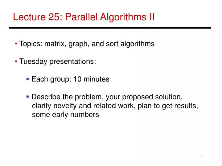
Lecture 25: Parallel Algorithms II. Topics: matrix, graph, and sort algorithms Tuesday presentations: Each group: 10 minutes Describe the problem, your proposed solution, clarify novelty and related work, plan to get results, some early numbers. Gaussian Elimination.

E N D
Lecture 25: Parallel Algorithms II • Topics: matrix, graph, and sort algorithms • Tuesday presentations: • Each group: 10 minutes • Describe the problem, your proposed solution, • clarify novelty and related work, plan to get results, • some early numbers
Gaussian Elimination • Solving for x, where Ax=b and A is a nonsingular matrix • Note that A-1Ax = A-1b = x ; keep applying transformations • to A such that A becomes I ; the same transformations • applied to b will result in the solution for x • Sequential algorithm steps: • Pick a row where the first (ith) element is non-zero and normalize the row so that the first (ith) element is 1 • Subtract a multiple of this row from all other rows so that their first (ith) element is zero • Repeat for all i
Sequential Example 2 4 -7 x1 3 3 6 -10 x2 = 4 -1 3 -4 x3 6 1 2 -7/2 x1 3/2 3 6 -10 x2 = 4 -1 3 -4 x3 6 1 2 -7/2 x1 3/2 0 0 1/2 x2 = -1/2 -1 3 -4 x3 6 1 2 -7/2 x1 3/2 0 0 1/2 x2 = -1/2 0 5 -15/2 x3 15/2 1 2 -7/2 x1 3/2 0 5 -15/2 x2 = 15/2 0 0 1/2 x3 -1/2 1 2 -7/2 x1 3/2 0 1 -3/2 x2 = 3/2 0 0 1/2 x3 -1/2 1 0 -1/2 x1 -3/2 0 1 -3/2 x2 = 3/2 0 0 1/2 x3 -1/2 1 0 -1/2 x1 -3/2 0 1 -3/2 x2 = 3/2 0 0 1 x3 -1 1 0 0 x1 -2 0 1 0 x2 = 0 0 0 1 x3 -1
Algorithm Implementation • The matrix is input in staggered form • The first cell discards inputs until it finds • a non-zero element (the pivot row) • The inverse r of the non-zero • element is now sent rightward • r arrives at each cell at the same • time as the corresponding • element of the pivot row
Algorithm Implementation • Each cell stores di = r ak,I – the value for the normalized pivot row • This value is used when subtracting a multiple of the pivot row from other rows • What is the multiple? It is aj,1 • How does each cell receive aj,1 ? It is passed rightward by the first cell • Each cell now outputs the new values for each row • The first cell only outputs zeroes and these outputs are no longer needed
Algorithm Implementation • The outputs of all but the first cell must now go through the remaining • algorithm steps • A triangular matrix of processors efficiently implements the flow of data • Number of time steps? • Can be extended to compute the inverse of a matrix
Implementation on 2d Processor Array Row 3 Row 2 Row 1 Row 3 Row 2 Row 3 Row 1 Row 1/2 Row 1/3 Row 1 Row 2 Row 2/3 Row 2/1 Row 2 Row 3 Row 3/1 Row 3/2 Row 3 Row 1 Row 2 Row 1 Row 3 Row 2 Row 1
Algorithm Implementation • Diagonal elements of the processor array can broadcast • to the entire row in one time step (if this assumption is not • made, inputs will have to be staggered) • A row sifts down until it finds an empty row – it sifts down • again after all other rows have passed over it • When a row passes over the 1st row, the value of ai1 is • broadcast to the entire row – aij is set to 1 if ai1 = a1j = 1 • – in other words, the row is now the ith row of A(1) • By the time the kth row finds its empty slot, it has already • become the kth row of A(k-1)
Algorithm Implementation • When the ith row starts moving again, it travels over • rows ak (k > i) and gets updated depending on • whether there is a path from i to j via vertices < k (and • including k)
Shortest Paths • Given a graph and edges with weights, compute the • weight of the shortest path between pairs of vertices • Can the transitive closure algorithm be applied here?
Shortest Paths Algorithm The above equation is very similar to that in transitive closure
Sorting with Comparison Exchange • Earlier sort implementations assumed processors that • could compare inputs and local storage, and generate • an output in a single time step • The next algorithm assumes comparison-exchange • processors: two neighboring processors I and J (I < J) • show their numbers to each other and I keeps the • smaller number and J the larger
Odd-Even Sort • N numbers can be sorted on an N-cell linear array • in O(N) time: the processors alternate operations with • their neighbors
Shearsort • A sorting algorithm on an N-cell square matrix that • improves execution time to O(sqrt(N) logN) • Algorithm steps: • Odd phase: sort each row with odd-even sort (all odd • rows are sorted left to right and all even • rows are sorted right to left) • Even phase: sort each column with odd-even sort • Repeat • Each odd and even phase takes O(sqrt(N)) steps – the • input is guaranteed to be sorted in O(logN) steps
The 0-1 Sorting Lemma If a comparison-exchange algorithm sorts input sets consisting solely of 0’s and 1’s, then it sorts all input sets of arbitrary values
Complexity Proof • How do we prove that the algorithm completes in O(logN) • phases? (each phase takes O(sqrt(N)) steps) • Assume input set of 0s and 1s • There are three types of rows: all 0s, all 1s, and mixed • entries – we will show that after every phase, the number • of mixed entry rows reduces by half • The column sort phase is broken into the smaller steps • below: move 0 rows to the top and 1 rows to the bottom; • the mixed rows are paired up and sorted within pairs; • repeat these small steps until the column is sorted
Example • The modified algorithm will behave as shown below: • white depicts 0s and blue depicts 1s
Proof • If there are N mixed rows, we are guaranteed to have • fewer than N/2 mixed rows after the first step of the • column sort (subsequent steps of the column sort may • not produce fewer mixed rows as the rows are not sorted) • Each pair of mixed rows produces at least one pure row • when sorted