S077: Applied Longitudinal Data Analysis Week #3: What Topics Are Covered In Today’s Overview?

1. S077: Applied Longitudinal Data AnalysisWeek #3: What Topics Are Covered In Today’s Overview?

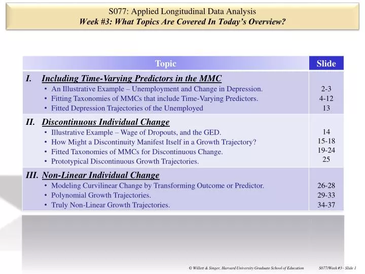
2. S077: Applied Longitudinal Data AnalysisI. Time-Varying Predictors: Illustrative Example • Sample: 254 people identified at unemployment offices. • Design: Goal was to collect 3 waves of data per person at 1, 5 &11 months after job loss. In reality, though, data set is not time-structured: • Interview 1 was within 1 day & 2 months of job loss. • Interview 2 was between 3 & 8 months of job loss. • Interview 3 was between 10 & 16 months of job loss. • In addition, not everyone completed 2nd & 3rd interview. • Outcome: Depression measured on the CES-D scale: • Twenty 4-point items (possible score ranged from 0 to 80). • Time-Varying Predictor: Unemployment status (UNEMP) • 132 were unemployed at every interview. • 61 were always working after first interview. • 41 were still unemployed at second interview, but working by third. • 19 were working at second interview, but were unemployed again by third. • Research Question: • How does unemployment affect the symptomatology of depression, over time? Source: Liz Ginexi and colleagues (2000), Journal of Occupational Health Psychology. (ALDA, Section 5.3..1, pp160-161)

3. UNEMP (by design, must be 1 at wave 1) TIME = MONTHSsince job loss ID 7589 has 3 waves, all unemployed ID 65641 has 3 waves, re-employed after 1st wave ID 53782 has 3 waves, re-employed at 2nd, unemployed again at 3rd S077: Applied Longitudinal Data AnalysisI. What Does A Person-Period Dataset Look Like, When It Contains Time-Varying Predictors? How Shall We Proceed? What Multilevel Models for Change Must We Fit, To Address the Research Question? (ALDA, Table 5.6, p161)

4. Level-1 Model: Level-2 Model:  How can it go in at Level-2? Composite Model:  But, it looks like we could just stick it in here? On the first day of job loss, the average person has an estimated CES-D of 17.7 On average, CES-D declines by 0.42/mo There’s statistically significant within-person residual variation. Where do we add time-varying predictor UNEMP? There’s statistically significant variation in initial status and rates of change. S077: Applied Longitudinal Data AnalysisI. Model A– Ignoring the Time-Varying Predictor &Fitting an Unconditional Growth Model Let’s just get a sense of the data by ignoring UNEMP, and first fitting the usual unconditional growth model (ALDA, Section 5.3.1, pp 159-164)

5. Logical impossibility? Population average rate of change in CES-D, controlling for UNEMP. Population average difference, over time, in CES-D by UNEMPstatus. Remains unemployed CES-D 20 Reemployed at 5 months Unemployed again at 10 Reemployed at 10 months Reemployed at 5 months CES-D CES-D CES-D 20 20 20 15 g20 g20 15 15 15 g20 g20 10 10 10 10 5 0 2 4 6 8 10 12 14 Months since job loss 5 5 5 0 2 4 6 8 10 12 14 0 2 4 6 8 10 12 14 0 2 4 6 8 10 12 14 Months since job loss Months since job loss Months since job loss S077: Applied Longitudinal Data AnalysisI. Model B -- Add the Time-Varying Predictor into the Composite Specification Directly? How Can We Understand This Graphically? Although the magnitude of the time-varying predictor’s effect remains constant, the time-varying nature of UNEMP’s values implies the existence of many possible true individual trajectories, such as: What Happens When We Fit This Model To Our Data? (ALDA, Section 5.3.1, pp 159-164)

6. Look what happens to folk who get a job!!! Monthly rate of decline is cut in half by controlling for UNEMP (still stat. sig.) UNEMP has a large and stat. sig. effect. Model Bis a better fit (difference in deviance = 25.5, 1 df, p<.001) CES-D 20 Consistently Unemployed (UNEMP=1): UNEMP = 1 15 10 UNEMP = 0 Consistently Employed (UNEMP=0): 5 0 2 4 6 8 10 12 14 Months since job loss S077: Applied Longitudinal Data AnalysisI. Fitting & Interpreting Model B, Which Now Contains Time-Varying Predictor UNEMP What about the variance components? (ALDA, Section 5.3.1, pp. 162-167)

7. Look what happened to the Level-2 VC’s • In this example, they’ve increased! • Why? Because including a time-varying predictor changes the meaning of the individual growth parameters (e.g., intercept now refers to value of the outcome when all level-1 predictors, including UNEMP are 0). • Level-1 VC, • Adding UNEMP to the unconditional growth model (A) reduces its magnitude 68.85 to 62.39. • UNEMP predicts 9.4% of the variation in CES-D scores. S077: Applied Longitudinal Data AnalysisI. Careful -- Variance Components Can Be Weird When You Add Time-Varying Predictors When including time-invariant predictors in the model, we already understand which variance components will differ and how: • Level-1 Variance Componentswill remain relatively stable because time-invariant predictors cannot predict (much of) the within-person variation. • Level-2 Variance Componentswill decline if the time-invariant predictors successfully predict some of the between-person variation. When including time-varying predictors, all the variance components can change, but • Although you can continue to interpret a model-to-model decrease in the magnitude of the level-1 variance components meaningfully, … •  Changes in the level-2 variance components may not appear to make sense!!! We can clarify what’s happened by decomposing the composite specification back into a level 1/level-2 representation … (ALDA, Section 5.3.1, pp. 162-167)

8. Unlike time-invariant predictors, time-varying predictors are entered into the level-1 model. Level-1 Model: Level-2 Models: • But, notice that … in Model B: • The level-2 model for 2i has no residual! • The value of 2ihas effectively been “fixed” – to the same hypothesized value – for everyone in the population. • So, the model is implicitly hypothesizing that there is no stochastic variation across people in this parameter. S077: Applied Longitudinal Data AnalysisI. A Clue! Decomposing the Composite Specification of Model B Into Its L1/L2 Specification • But, Is this reasonable? • Should we really assume that the effect of the person-specific predictor is identical across people? • No, with a little thought, we can try to relax the assumption  (ALDA, Section 5.3.1, pp. 168-169)

9. You can allow the effect of UNEMP to differ randomly across people in the pop by adding in a level-2 residual. • Check your software to make sure you know what you’re doing … Level-2 Models: Level-1 Model: • But, you may not be able to afford the cost: • Adding this residual adds 3 new variance components. • If you have only a few waves of data, you may be straining the resources of your data . • Here, we can’t actually fit this model!! S077: Applied Longitudinal Data AnalysisI. Adding the “Omitted” Level-2 Stochastic Variation in the Effect of UNEMP • Moral: Themultilevel model for change can easily handle time-varying predictors, but… • Think carefully about the consequences for both the structural and stochastic parts of the model. • Don’t just “buy” the default specification in your software. • Until you’re sure you know what you’re doing, always write out your model in both the composite and L1/L2 specifications before specifying code to a computer package. So … Are we happy with Model B as the “final” model??? Is there any other way to allow the effect of UNEMP to vary – if not across people, across TIME? (ALDA, Section 5.3.1, pp. 169-171)

10. Because of the way in which we’ve constructed the models with time-varying predictors, we’ve automatically constrained UNEMP to have only a “main effect” on the trajectory’s elevation. When analyzing the effects of time-invariant predictors, we automatically allowed predictors to affect the trajectory’s slope ... • Two possible (equivalent) interpretations: • The effect of UNEMP differs across occasions. • The rate of change in depression differs by unemployment status. • But you need to think very carefully about the hypothesized error structure: • We’ve added another level-1 parameter to represent the interaction. • Just like we asked about the main effect of time-varying predictor UNEMP, perhaps we should allow the interaction effect also to differ stochastically across people in the pop? • We won’t right now, but soon ... S077: Applied Longitudinal Data AnalysisI. Model C: What If the Effect of a Time-Varying Predictor Differs Over Time? To allow the effect of a time-varying predictor to differ over time, just add its interaction with TIME … What happens when we fit this model to data? (ALDA, Section 5.3.2, pp. 171-172)

11. Main effect of TIME is now positive (!) & not stat sig ?!?!?!?!?!?!?!?! UNEMP×TIMEinteraction is stat sig (p<.05). Model C is a better fit than Model B ( Deviance = 4.6, 1 df, p<.05). What about people who get a job? Consistently unemployed (UNEMP=1) Consistently employed (UNEMP=0) • S077: Applied Longitudinal Data AnalysisI. Model C: What If the Effect of a Time-Varying Predictor Differs Over Time? Perhaps we should constrain the slope of the trajectory for the reemployed to be zero? (ALDA, Section 5.3.2, pp. 171-172)

12. Should we remove the main effect of TIME? (which is the slope when UNEMP=0)  Yes, but this creates a lack of congruence between the model’s fixed and stochastic parts So, let’s better align the parts by having UNEMP*TIME be both fixed and random  If we’re allowing the UNEMP*TIME slope to differ randomly across people, might we also need to allow the effect of UNEMP itself to do the same? Model D: UNEMP has both a fixed & random effect UNEMP*TIME has both a fixed & random effect S077: Applied Longitudinal Data AnalysisI. Model D: Constraining the Slope of the Individual Growth Trajectory for the Re-Employed? What happens when we fit this model to data? (ALDA, Section 5.3.2, pp. 172-173)

13. Consistently unemployed Consistently employed What about people who get a job? Best fitting model S077: Applied Longitudinal Data AnalysisI: Model D: Constraining Slope of the Individual Growth Trajectory for the Re-Employed? (ALDA, Section 5.3.2, pp. 172-173)

14. S077: Applied Longitudinal Data AnalysisII. Modeling Discontinuous Individual Change: IllustrativeExample • Sample: 888 male high school dropouts, from an earlier analysis. • Research Design: • Each was interviewed between 1 and 13 times after dropping out. • 34.6% (n=307) earned a GED at some point during data collection. • OLD Research Questions: • How do log(WAGES) change over time? • Do wage trajectories differ by ethnicity and highest grade completed? • NEW Research Questions: What is the effect of GED attainment? Does earning a GED: • affect the wage trajectory’s elevation? • affect the wage trajectory’s slope? • create a discontinuity in the wage trajectory? Data source: Murnane, Boudett and Willett (1999), Evaluation Review (ALDA, Section 6.1.1, pp 190-193)

15. F: Immediate shifts in both elevation & rate of change LNW 2.5 D: An immediate shift in rate of change; no difference in elevation GED B: An immediate shift in elevation; no difference in rate of change 2.0 A: No effect of GED whatsoever 1.5 0 2 4 6 8 10 EXPER S077: Applied Longitudinal Data AnalysisII. Theory: How Might GED Receipt Affect an Individual’s Wage Trajectory? Let’s start by considering four plausible effects of GED receipt by imagining what the wage trajectory might look like for someone who got a GED 3 years after labor force entry (post dropout) How do we represent trajectories like these within the context of a linear growth model???  (ALDA, Figure 6.1, p 193)

16. Post-GED (GED=1): Pre-GED (GED=0): • S077: Applied Longitudinal Data AnalysisII. Trajectory B: Including a Discontinuity in Elevation, and Not In Slope Key Idea: It’s easy; simply include GED as a time-varying effect at level-1 … (ALDA, Section 6.1.1, pp 194-195)

17. Post-GED (POSTEXP clocked in same cadence as EXPER): Pre-GED (POSTEXP=0): • POSTEXPij • A new time-varying predictor that clocks “TIME since GED receipt” (in the same cadence as EXPER). • Equals 0 prior to GED. • After GED is received, it counts“Post GEDexperience.” • S077: Applied Longitudinal Data AnalysisII. Trajectory D: Including a Discontinuity in Slope, and Not in Elevation (ALDA, Section 6.1.1, pp 195-198)

18. Post-GED Pre-GED • S077: Applied Longitudinal Data AnalysisII. Trajectory F: Including Discontinuities In Both Elevation and Slope Now, let’s try fitting all these models … (ALDA, Section 6.1.1, pp 195-198)

19. (UERATE-7) is the local area unemployment rate(a time-varying control predictor), centered around 7% for interpretability Benchmark against which we will compare the discontinuous models -7 4 random effects 5 fixed effects S077: Applied Longitudinal Data AnalysisII. Let’s Start By Fitting a “Baseline Model” In Which There Are No Discontinuities To compare this deviance statistic to more complex models appropriately , we need to know how many parameters have been estimated to achieve this value of deviance. (ALDA, Section 6.1.2, pp 201-202)

20. specific terms in the model deviance statistic (for model comparison) n parameters (for d.f.) Baseline just shown S077: Applied Longitudinal Data AnalysisII. Now, What’s the Best Way to Proceed … ? Instead of constructing tables of (seemingly endless) parameter estimates, we’re going to construct a summary table that presents the… (ALDA, Section 6.1.2, pp 202-203)

21. B: Add GED as both a fixed and random effect (1 extra fixed parameter; 3 extra random) Deviance=25.0, 4 df, p<.001—keep GED effect C: But, does the GED discontinuity differ across people? (do we need to keep the extra variance components for the effect of GED?) Deviance=12.8, 3 df, p<.01— keep variance components. S077: Applied Longitudinal Data AnalysisII. First Steps: Investigating A Potential Discontinuity in Elevation by Adding Effect of GED What about adding the discontinuity in slope? (ALDA, Section 6.1.2, pp 202-203)

22. S077: Applied Longitudinal Data AnalysisII. Next Steps: Investigating a Discontinuity in Slope by Adding the Effect of POSTEXP D: Adding POSTEXP as both a fixed and random effect (1 extra fixed parameter; 3 extra random) Deviance=13.1, 4 df, p<.05— keep POSTEXP effect E: But does the POSTEXP slope differ across people? (do we need to keep the extra variance components for the effect of POSTEXP?) Deviance=3.3, 3 df, ns—don’t need the POSTEXP random effects (but in comparison with A still need POSTEXP fixed effect) What if we include both types of discontinuity? (ALDA, Section 6.1.2, pp 203-204)

23. F: Add GED and POSTEXP simultaneously (each as both fixed and random effects) S077: Applied Longitudinal Data AnalysisII. Examining The Addition of Elevation and Slope Discontinuities Simultaneously comp. with B shows importance of POSTEXP comp. with D shows Importance of GED (ALDA, Section 6.1.2, pp 204-205)

24. S077: Applied Longitudinal Data AnalysisII. Can We Simplify by Eliminating theVariance Components for POSTEXP or GED? Each results in a worse fit, suggesting that Model F (which includes both random effects) is better (even though Model E suggested we might be able to eliminate the variance component for POSTEXP) We actually fit several other possible models (see ALDA) but Model Fwas the best alternative—so…how do we display its results? (ALDA, Section 6.1.2, pp 204-205)

25. Race • At dropout, no racial differences in wages. • Racial disparities increase over time because wages for Blacks increase at a slower rate. LNW White/ Latino earned a GED Black • Highest grade completed • Those who stay longer have higher initial wages. • This differential remains constant over time. • GED receipt has two effects • Upon GED receipt, wages rise immediately by 4.2%. • Post-GED receipt, wages rise annually by 5.2% (vs. 4.2% pre-receipt). S077: Applied Longitudinal Data AnalysisII. Displaying Fitted Growth Trajectories for Prototypical HS Dropouts 12th grade dropouts 9th grade dropouts (ALDA, Section 6.1.2, pp 204-206)

26. Earlier, we modeled ALCUSE, an outcome that we formed by taking the square root of the researchers’ original alcohol use measurement We can ‘de-transform’ the findings and return to the original scale, by squaring the predicted values of ALCUSE and re-plotting S077: Applied Longitudinal Data AnalysisIII: Modeling Non-Linear Change Using Transformations When facing obviously non-linear trajectories, we begin by trying transformation: • A straight line—even on a transformed scale—is a simple form with easily interpretable parameters. • Since many outcome metrics are ad hoc, transformation to another ad hoc scale may sacrifice little. Prototypical Individual Growth Trajectories Are Now Non-linear: By transforming the outcome before analysis, we have effectively modeled non-linear change over time. So … How do we know which variable to transform, using which transformation… ? (ALDA, Section 6.2, pp 208-210)

27. Step 1: What kinds of transformations do we consider? • Step 2: How do we know when to use which transformation? • Plot empirical growth trajectories. • Find linearizingtransformations by moving “up” or “down” in the direction of the “Bulge.” expand scale Generic variable V compress scale S077: Applied Longitudinal Data AnalysisIII. The “Rule of the Bulge” and the “Ladder of Transformations” (ALDA, Section 6.2.1, pp. 210-212)

28. Up in IQ Down in TIME S077: Applied Longitudinal Data AnalysisIII. Transforming the Growth Trajectory of a Single Child in the Berkeley Growth Study How Else Might We Model Non-linear Change? (ALDA, Section 6.2.1, pp. 211-213)

29. Polynomial of the “zero order” (because TIME0=1): • Like including a constant predictor 1 in the level-1 model. • Intercept represents vertical elevation. • Different people can have different elevations. • Polynomial of the “first order” (because TIME1=TIME): • Familiar individual growth model. • Varying intercepts and slopes yield criss-crossing lines. • Second order polynomial for quadratic change: • Includes both TIME and TIME2. • 0i = intercept (but now both TIME& TIME2 are 0). • 1i = instantaneous rate of change when TIME=0 (there is no longer a constant slope). • 2i = curvature parameter; larger its value, more dramatic its effect. • Peak is called a “stationary point”— a quadratic has only one. • Third order polynomial for cubic change: • Includes TIME, TIME2 and TIME3. • Can keep on adding other powers of TIME. • Each extra term adds another stationary point—cubic has two. S077: Applied Longitudinal Data AnalysisIII. Representing Non-Linear Individual Change by a Polynomial Function of Time (ALDA, Section 6.3.1, pp. 213-217)

30. S077: Applied Longitudinal Data AnalysisIII. Change as a Polynomial Function of Time: Illustrative Example • Sample: 45 boys & girls identified in 1st grade. Goal was to study behavior changes over time (until 6th grade) • Research Design: • At the end of every school year, teachers rated each child’s level of externalizing behavior using Achenbach’s Child Behavior Checklist: • 3 point scale (0=rarely/never; 1=sometimes; 2=often). • 24 aggressive, disruptive, or delinquent behaviors. • Outcome: • EXTERNAL — ranges from 0 to 68 (simple sum of scores). • Question Predictor: • FEMALE. • Research Question: • How does children’s level of externalizing behavior change over time? • Do trajectories of change differ for boys and girls? Source: Margaret Keileyet al. (2000) J. of Abnormal Child Psychology (ALDA, Section 6.3.2, p. 217)

31. Quadratic change (but with varying curvatures) Linear decline (at least until 4th grade) Little change over time (flat line?) Two stationary points? (suggests a cubic) Three stationary points? (suggests a quartic!!!) S077: Applied Longitudinal Data AnalysisIII. Selecting a Suitable Polynomial Trajectory for Individual Change? When faced with so many different patterns, how do you select a commonpolynomial for analysis? (ALDA, Section 6.3.2, pp 217-220)

32. Second impression: Maybe these ad hoc decisions aren’t the best? Quadratic? Would a quadratic do? S077: Applied Longitudinal Data AnalysisIII. Examining Possible Polynomial Trajectories, Using Exploratory OLS Methods First impression: Most fitted trajectories provide a reasonable summary for each child’s data Third realization: We need a common polynomial across all cases (and might the quartic be just too complex)? Using sample data to draw conclusions about the shape of the underlying true trajectories is tricky—let’s compare alternative models  (ALDA, Section 6.3.2, pp 217-220)

33. Add polynomial functions of TIME to person period data set Compare goodness of fit (accounting for all the extra parameters that get estimated) A: stat significant between- and within-child variation D: still no fixed effects for TIME terms, but now var comps are ns also Deviance=11.1, 5df, ns B: no fixed effect of TIME but stat sig var comps Deviance=18.5, 3df, p<.01 C: no fixed effects of TIME & TIME2 but stat sig var comps Deviance=16.0, 4df, p<.01 • S077: Applied Longitudinal Data AnalysisIII. Using Model-to-Model Comparisons To Test Higher-Order Polynomial Terms Quadratic (C) is best choice—and it turns out there are no gender differentials at all. (ALDA, Section 6.3.3, pp 220-223)

34. S077: Applied Longitudinal Data AnalysisIII. Truly Non-Linear Individual Change: Illustrative Example • Sample: 17 1st and 2nd graders • During a three week period, Terry repeatedly played a two-person checkerboard game called Fox ‘n Geese, with participants (hopefully) learning from experience: • Fox is controlled by the experimenter, at one end of the board. • Children have four geese, that they use to try to trap the fox. • Great for studying cognitive development because: • There exists a strategy that children can learn that will guarantee victory. • This strategy is not immediately obvious to children. • Many children can deduce the strategy over time . • Research Design: • Each child played up to 27 games (each game is a “wave”). • Outcome, NMOVES is the number of moves made by the child before making a catastrophic error (guaranteeing defeat)—ranges from 1 to 20. • Research Question: • How does the child’s success change over time? • What is the impact of a child’s reading (or cognitive) ability — READ (score on a standardized reading test) – on the change trajectory. Data source: Terry Tivnan (1980) Doctoral Dissertation, HGSE (ALDA, Section 6.4.1, pp. 224-225)

35. A lower asymptote, because everyone makes at least 1 move and it takes a while to figure out what’s going on An upper asymptote, because a child can make only a finite # moves each game Asmooth curve joining the asymptotes, that initially accelerates and then decelerates S077: Applied Longitudinal Data AnalysisIII. Selecting a Truly Non-Linear Trajectory for Individual Change These three features suggest a level-1 logistic change trajectorywhich, unlike our previous growth models, is non-linear in the individual growth parameters. (ALDA, Section 6.4.2, pp. 225-228)

36. Upper asymptote in this particular model is constrained to be 20 (1+19) 0i is related to, and determines, the intercept 1i determines the rapidity with which the trajectory approaches the upper asymptote When 1i is large, the trajectory rises more rapidly When 1i is small, the trajectory rises slowly (often not reaching an asymptote) Higher the value of 0i, the lower the intercept S077: Applied Longitudinal Data AnalysisIII. Understanding the Logistic Individual Change Trajectory Models can be fit in usual way using provided your software can do it  (ALDA, Section 6.4.2, pp 226-230)

37. Begins low and rises smoothly and non-linearly Not statistically significant (note small n’s), but better READers approach asymptote more rapidly S077: Applied Longitudinal Data AnalysisIII. Investigating Systematic Inter-Individual Differences in Logistic Change (ALDA, Section 6.4.2, pp 229-232)