Download
1 / 27
270 likes | 333 Views
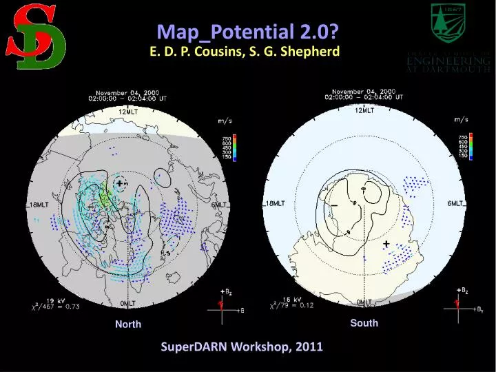
Map_Potential 2.0?. E. D. P. Cousins, S. G. Shepherd. South. North. SuperDARN Workshop, 2011. Map_Potential Procedure. Find Heppner Maynard boundary Get IMF values Add statistical model vectors Do spherical harmonic fit (SHF). Map_Potential Procedure.

E N D
Map_Potential 2.0? E. D. P. Cousins, S. G. Shepherd South North SuperDARN Workshop, 2011
Map_Potential Procedure • Find Heppner Maynard boundary • Get IMF values • Add statistical model vectors • Do spherical harmonic fit (SHF)
Map_Potential Procedure • Find Heppner Maynard boundary • Get IMF values • Add statistical model vectors • Do spherical harmonic fit (SHF)
Map_Potential Procedure • Find Heppner Maynard boundary • Get IMF values • Add statistical model vectors • Do spherical harmonic fit (SHF)
Map_Potential Procedure • Find Heppner Maynard boundary • Get IMF values • Add statistical model vectors • Do spherical harmonic fit (SHF)
Updates • Magnetic Field Model • Dipole → IGRF • Changes model vector calculation and SHF procedure • Statistical model data error weighting • Uniform → Variable • Changes SHF procedure • Statistical Model • RG96 → CS10 [Cousins and Shepherd, JGR, 2010] • Changes model vector calculation
Magnetic Field Model Dipole field IGRF field Difference 50° North -50° South
Magnetic Field Model North December 04, 2000 08:00 – 08:02 UT Dipole IGRF Difference 63 kV χ2/359=1.14 Over 72 hours: Average ΦPC Diff = 2% RMS Diff = 2kV 2%
Magnetic Field Model South December 04, 2000 08:00 – 08:02 UT Dipole IGRF Difference 60 kV χ2/267=2.00 Over 72 hours: Average ΦPC Diff = -4.5% RMS Diff = 1.6 kV -6%
Heppner Maynard Boundary South January 05, 2004 03:20:00 – 03:20:22 UT Original No default HMB latitude • With no data: Original procedure sets HMB = 62° • New procedure uses model lower limit
Model Data Weighting North April 22, 2001 11:00 – 11:10 UT Org. Weighting New Weighting 89 kV χ2/107=1.74 • Model vector errors: • Original: dependent on order of fit and on average of data errors • New: Original value, scaled by number of data vectors in vicinity
Model Data Weighting North April 22, 2001 11:00 – 11:10 UT Org. Weighting New Weighting
Model Data Weighting North April 22, 2001 11:00 – 11:10 UT Org. Weighting New Weighting Difference 89 kV χ2/107=1.74 Average Difference over 24 hours < 1% 4%
Model Data Weighting South May 12, 2001 12:00 – 12:02 UT Org. Weighting New Weighting Difference 71 kV χ2/166=1.74 Average Difference over 24 hours ≈ 1% 3%
Statistical Model RG96 model Fit w/ RG96 North April 01, 2000 18:32 – 18:34 UT Difference 68 kV -34 38 Fit w/ CS10 CS10 model 15% Average Difference over 72 hours ≈ 1% (≈ 3% in summer ≈ -7% in winter)
Statistical Model RG96 model Fit w/ RG96 South March 06, 2000 06:00 – 06:10 UT Difference -43 19 Fit w/ CS10 CS10 model -22% • Average Difference over 72 hours ≈ -12% • (≈-7% in summer • ≈ -9% in winter) 62 kV
Total Difference North April 01, 2000 18:32 – 18:34 UT Original New Difference 87 kV χ2/300=1.95 By = -2.6 nT Bz = -10.7 nT Average Difference over 72 hours ≈ 3% Diff due to new model: 11 kV 15% 21%
Total Difference South March 06, 2000 06:00 – 06:10 UT Original New Difference 61 kV χ2/86=1.41 By = -5.7 nT Bz = -7.1nT Average Difference over 72 hours ≈ -8% Diff due to new model: -17 kV -22% -20%
Total Difference New Difference By, Bz = 0, -6.2 nT • Often little or no difference when data coverage is excellent
Total Difference -2.2 % -2.7 %
Total Difference 2.0 % -4.3 %
Total Difference 5.9 % -3.0 %
Summary • Magnetic Field Model: Dipole → IGRF • Statistical data error weighting: Uniform → Variable • Statistical Model: RG96 → CS10
Summary • Magnetic Field Model: Dipole → IGRF • Statistical data error weighting: Uniform → Variable • Statistical Model: RG96 → CS10 • Small (0 – 10%) average offset between new & old ΦPC • RMS difference between patterns is typically • 2-4 kV in North, 6-8 kV in South (mostly due to new model) • Up to 20 – 30% change in individual patterns’ ΦPC with moderate to low data coverage
Summary • Magnetic Field Model: Dipole → IGRF • Statistical data error weighting: Uniform → Variable • Statistical Model: RG96 → CS10 • Small (0 – 10%) average offset between new & old ΦPC • RMS difference between patterns is typically • 2-4 kV in North, 6-8 kV in South (mostly due to new model) • Up to 20 – 30% change in individual patterns’ ΦPC with moderate to low data coverage • Still needed: get IMF data from OMNI • More robust time shifting