Download
1 / 38

E N D
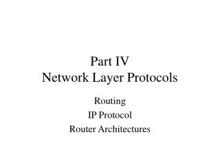
Topic 3Network LayerPart C The majority of the slides in this course are adapted from the accompanying slides to the books by Larry Peterson and Bruce Davie and by Jim Kurose and Keith Ross. Additional slides and/or figures from other sources and from Vasos Vassiliou are also included in this presentation. Network Layer
Introduction Virtual circuit and datagram networks Bridges, switches, hubs, etc. IP: Internet Protocol Datagram format IPv4 addressing IPv6 Routing algorithms and Protocols MPLS Topic 3: Network Layer Network Layer
routing algorithm local forwarding table header value output link 0100 0101 0111 1001 3 2 2 1 value in arriving packet’s header 1 0111 2 3 Interplay between routing and forwarding Network Layer
Routing Principles • Routing: delivering a packet to its destination on the best possible path • Routing steps: (a) determine node network address (b) compute/construct the path (c) forward the packet to destination Here, we will focus on (b) - routing alg. for path computation Network Layer
Routing Alg Requirements • Find path with min delay, cost or other metric • dynamic reconfiguration after failures/changes • adaptive load balancing Network Layer
5 3 5 2 2 1 3 1 2 1 x z w y u v Graph abstraction Graph: G = (N,E) N = set of routers = { u, v, w, x, y, z } E = set of links ={ (u,v), (u,x), (v,x), (v,w), (x,w), (x,y), (w,y), (w,z), (y,z) } Remark: Graph abstraction is useful in other network contexts Example: P2P, where N is set of peers and E is set of TCP connections Network Layer
5 3 5 2 2 1 3 1 2 1 x z w y u v Graph abstraction: costs • c(x,x’) = cost of link (x,x’) • - e.g., c(w,z) = 5 • cost could always be 1, or • inversely related to bandwidth, • or inversely related to • congestion Cost of path (x1, x2, x3,…, xp) = c(x1,x2) + c(x2,x3) + … + c(xp-1,xp) Question: What’s the least-cost path between u and z ? Routing algorithm: algorithm that finds least-cost path Network Layer
Global or decentralized? Global: all routers have complete topology, link cost info “link state” algorithms Decentralized: router knows physically-connected neighbors, link costs to neighbors iterative process of computation, exchange of info with neighbors “distance vector” algorithms Static or dynamic? Static: routes change slowly over time Dynamic: routes change more quickly periodic update in response to link cost changes Routing Algorithm classification Network Layer
Dijkstra’s algorithm net topology, link costs known to all nodes accomplished via “link state broadcast” all nodes have same info computes least cost paths from one node (‘source”) to all other nodes gives forwarding table for that node iterative: after k iterations, know least cost path to k dest.’s A Link-State Routing Algorithm Network Layer
Dijsktra’s Algorithm 1 Initialization: 2 N' = {u} 3 for all nodes v 4 if v adjacent to u 5 then D(v) = c(u,v) 6 else D(v) = ∞ 7 8 Loop 9 find w not in N' such that D(w) is a minimum 10 add w to N' 11 update D(v) for all v adjacent to w and not in N' : 12 D(v) = min( D(v), D(w) + c(w,v) ) 13 /* new cost to v is either old cost to v or known 14 shortest path cost to w plus cost from w to v */ 15 until all nodes in N' Network Layer
5 3 5 2 2 1 3 1 2 1 x z w u y v Dijkstra’s algorithm: example D(v),p(v) 2,u 2,u 2,u D(x),p(x) 1,u D(w),p(w) 5,u 4,x 3,y 3,y D(y),p(y) ∞ 2,x Step 0 1 2 3 4 5 N' u ux uxy uxyv uxyvw uxyvwz D(z),p(z) ∞ ∞ 4,y 4,y 4,y Network Layer
Algorithm complexity: n nodes each iteration: need to check all nodes, w, not in N n(n+1)/2 comparisons: O(n2) more efficient implementations possible: O(nlogn) Oscillations possible: e.g., link cost = amount of carried traffic A A A A D D D D B B B B C C C C 1 1+e 2+e 0 2+e 0 2+e 0 0 0 1 1+e 0 0 1 1+e e 0 0 0 e 1 1+e 0 1 1 e … recompute … recompute routing … recompute initially Dijkstra’s algorithm, discussion Network Layer
Distance vector algorithm Basic idea: • Each node periodically sends its own distance vector estimate to neighbors • When node a node x receives new DV estimate from neighbor, it updates its own DV using B-F equation: Dx(y) ← minv{c(x,v) + Dv(y)} for each node y ∊ N • Under minor, natural conditions, the estimate Dx(y) converge the actual least cost dx(y) Network Layer
Iterative, asynchronous: each local iteration caused by: local link cost change DV update message from neighbor Distributed: each node notifies neighbors only when its DV changes neighbors then notify their neighbors if necessary wait for (change in local link cost of msg from neighbor) recompute estimates if DV to any dest has changed, notify neighbors Distance Vector Algorithm (2) Each node: Network Layer
cost to x y z x 0 2 7 y from ∞ ∞ ∞ z ∞ ∞ ∞ 2 1 7 z x y Dx(z) = min{c(x,y) + Dy(z), c(x,z) + Dz(z)} = min{2+1 , 7+0} = 3 Dx(y) = min{c(x,y) + Dy(y), c(x,z) + Dz(y)} = min{2+0 , 7+1} = 2 node x table cost to cost to x y z x y z x 0 2 3 x 0 2 3 y from 2 0 1 y from 2 0 1 z 7 1 0 z 3 1 0 node y table cost to cost to cost to x y z x y z x y z x ∞ ∞ x 0 2 7 ∞ 2 0 1 x 0 2 3 y y from 2 0 1 y from from 2 0 1 z z ∞ ∞ ∞ 7 1 0 z 3 1 0 node z table cost to cost to cost to x y z x y z x y z x 0 2 7 x 0 2 3 x ∞ ∞ ∞ y y 2 0 1 from from y 2 0 1 from ∞ ∞ ∞ z z z 3 1 0 3 1 0 7 1 0 time Network Layer
1 4 1 50 x z y Distance Vector: link cost changes Link cost changes: • node detects local link cost change • updates routing info, recalculates distance vector • if DV changes, notify neighbors At time t0, y detects the link-cost change, updates its DV, and informs its neighbors. At time t1, z receives the update from y and updates its table. It computes a new least cost to x and sends its neighbors its DV. At time t2, y receives z’s update and updates its distance table. y’s least costs do not change and hence y does not send any message to z. “good news travels fast” Network Layer
60 4 1 50 x z y Distance Vector: link cost changes Link cost changes: • good news travels fast • bad news travels slow - “count to infinity” problem! • 44 iterations before algorithm stabilizes: see text Poissoned reverse: • If Z routes through Y to get to X : • Z tells Y its (Z’s) distance to X is infinite (so Y won’t route to X via Z) • will this completely solve count to infinity problem? Network Layer
Message complexity LS: with n nodes, E links, O(nE) msgs sent DV: exchange between neighbors only convergence time varies Speed of Convergence LS: O(n2) algorithm requires O(nE) msgs may have oscillations DV: convergence time varies may be routing loops count-to-infinity problem Robustness: what happens if router malfunctions? LS: node can advertise incorrect link cost each node computes only its own table DV: DV node can advertise incorrect path cost each node’s table used by others error propagate thru network Comparison of LS and DV algorithms Network Layer
scale: with 200 million destinations: can’t store all dest’s in routing tables! routing table exchange would swamp links! administrative autonomy internet = network of networks each network admin may want to control routing in its own network Hierarchical Routing Our routing study thus far - idealization • all routers identical • network “flat” … not true in practice Network Layer
Routing in the Internet • The Global Internet consists of Autonomous Systems (AS) interconnected with eachother: • Stub AS: small corporation • Multihomed AS: large corp. (no transit) • Transit AS: provider • Two level routing: • Intra-AS: administrator is responsible for choice • Inter-AS: unique standard Network Layer
aggregate routers into regions, “autonomous systems” (AS) routers in same AS run same routing protocol “intra-AS” routing protocol routers in different AS can run different intra-AS routing protocol Gateway router Direct link to router in another AS Hierarchical Routing Network Layer
Forwarding table is configured by both intra- and inter-AS routing algorithm Intra-AS sets entries for internal dests Inter-AS & Intra-As sets entries for external dests 3a 3b 2a AS3 AS2 1a 2c AS1 2b 3c 1b 1d 1c Inter-AS Routing algorithm Intra-AS Routing algorithm Forwarding table Interconnected ASes Network Layer
AS1 needs: to learn which dests are reachable through AS2 and which through AS3 to propagate this reachability info to all routers in AS1 Job of inter-AS routing! Suppose router in AS1 receives datagram for which dest is outside of AS1 Router should forward packet towards on of the gateway routers, but which one? 3a 3b 2a AS3 AS2 1a AS1 2c 2b 3c 1b 1d 1c Inter-AS tasks Network Layer
Example: Setting forwarding table in router 1d • Suppose AS1 learns from the inter-AS protocol that subnet x is reachable from AS3 (gateway 1c) but not from AS2. • Inter-AS protocol propagates reachability info to all internal routers. • Router 1d determines from intra-AS routing info that its interface I is on the least cost path to 1c. • Puts in forwarding table entry (x,I). Network Layer
Determine from forwarding table the interface I that leads to least-cost gateway. Enter (x,I) in forwarding table Use routing info from intra-AS protocol to determine costs of least-cost paths to each of the gateways Learn from inter-AS protocol that subnet x is reachable via multiple gateways Hot potato routing: Choose the gateway that has the smallest least cost Example: Choosing among multiple ASes • Now suppose AS1 learns from the inter-AS protocol that subnet x is reachable from AS3 and from AS2. • To configure forwarding table, router 1d must determine towards which gateway it should forward packets for dest x. • This is also the job on inter-AS routing protocol! • Hot potato routing: send packet towards closest of two routers. Network Layer
Intra-AS Routing • Also known as Interior Gateway Protocols (IGP) • Most common Intra-AS routing protocols: • RIP: Routing Information Protocol • OSPF: Open Shortest Path First • IGRP: Interior Gateway Routing Protocol (Cisco proprietary) Network Layer
RIP ( Routing Information Protocol) • Distance vector algorithm • Included in BSD-UNIX Distribution in 1982 • Distance metric: # of hops (max = 15 hops) • Distance vectors: exchanged among neighbors every 30 sec via Response Message (also called advertisement) • Each advertisement: list of up to 25 destination nets within AS Network Layer
routed routed RIP Table processing • RIP routing tables managed by application-level process called route-d (daemon) • advertisements sent in UDP packets, periodically repeated Transprt (UDP) Transprt (UDP) network forwarding (IP) table network (IP) forwarding table link link physical physical Network Layer
OSPF (Open Shortest Path First) • “open”: publicly available • Uses Link State algorithm • LS packet dissemination • Topology map at each node • Route computation using Dijkstra’s algorithm • OSPF advertisement carries one entry per neighbor router • Advertisements disseminated to entire AS (via flooding) • Carried in OSPF messages directly over IP (rather than TCP or UDP Network Layer
OSPF “advanced” features (not in RIP) • Security: all OSPF messages authenticated (to prevent malicious intrusion) • Multiple same-cost paths allowed (only one path in RIP) • For each link, multiple cost metrics for different TOS (e.g., satellite link cost set “low” for best effort; high for real time) • Integrated uni- and multicast support: • Multicast OSPF (MOSPF) uses same topology data base as OSPF • Hierarchical OSPF in large domains. Network Layer
Hierarchical OSPF • Two-level hierarchy: local area, backbone. • Link-state advertisements only in area • each nodes has detailed area topology; only know direction (shortest path) to nets in other areas. • Area border routers:“summarize” distances to nets in own area, advertise to other Area Border routers. • Backbone routers: run OSPF routing limited to backbone. • Boundary routers: connect to other AS’s. Network Layer
Internet inter-AS routing: BGP • BGP (Border Gateway Protocol):the de facto standard • BGP provides each AS a means to: • Obtain subnet reachability information from neighboring ASs. • Propagate the reachability information to all routers internal to the AS. • Determine “good” routes to subnets based on reachability information and policy. • Allows a subnet to advertise its existence to rest of the Internet: “I am here” Network Layer
Why different Intra- and Inter-AS routing ? Policy: • Inter-AS: admin wants control over how its traffic routed, who routes through its net. • Intra-AS: single admin, so no policy decisions needed Scale: • hierarchical routing saves table size, reduced update traffic Performance: • Intra-AS: can focus on performance • Inter-AS: policy may dominate over performance Network Layer
Multiple constraints QoS Routing Given: - a (real time) connection request with specified QoS requirements (e.g., Bdw, Delay, Jitter, packet loss, path reliability etc) Find: - a min cost (typically min hop) path which satisfies such constraints - if no feasible path found, reject the connection Network Layer
Example of QoS Routing D = 25, BW = 55 D = 30, BW = 20 A B D = 5, BW = 90 D = 14, BW = 90 D = 5, BW = 90 D = 5, BW = 90 D = 2, BW = 90 D = 1, BW = 90 D = 5, BW = 90 D = 3, BW = 105 Constraints: Delay (D) <= 25, Available Bandwidth (BW) >= 30 Network Layer
2 Hop Path --------------> Fails (Total delay = 55 > 25 and Min. BW = 20 < 30)3 Hop Path ----------> Succeeds!! (Total delay = 24 < 25, and Min. BW = 90 > 30)5 Hop Path ----------> Do not consider, although (Total Delay = 16 < 25, Min. BW = 90 > 30) D = 25, BW = 55 D = 30, BW = 20 A B D = 5, BW = 90 D = 14, BW = 90 D = 5, BW = 90 D = 5, BW = 90 D = 2, BW = 90 D = 1, BW = 90 D = 5, BW = 90 D = 3, BW = 105 Constraints: Delay (D) <= 25, Available Bandwidth (BW) >= 30 We look for feasible path with least number of hops Network Layer
Benefits of QoS Routing • Without QoS routing: • must probe path & backtrack; non optimal path, control traffic and processing OH, latency With QoS routing: • optimal route; “focused congestion” avoidance • more efficient Call Admission Control (at the source) • more efficient bandwidth allocation (per traffic class) • resource renegotiation easier Network Layer
The components of QoS Routing • Q-OSPF: link state based protocol; it disseminates link state updates (including QoS parameters) to all nodes; it creates/maintains global topology map at each node • Bellman-Ford constrained path computation algorithm: it computes constrained min hop paths to all destinations at each node based on topology map • (Call Acceptance Control) • Packet Forwarding: source route or MPLS Network Layer