Download
1 / 10
100 likes | 222 Views
ELF.01.5 – The Logarithmic Function – Graphic Perspective. MCB4U - Santowski. (A) Graph of Logarithmic Functions. Graph the exponential function f(x) = 2 x and then graph the inverse y = f -1 (x) which is x = 2 y . This inverse is called a logarithm and is written as y = log 2 (x)

E N D
ELF.01.5 – The Logarithmic Function – Graphic Perspective MCB4U - Santowski
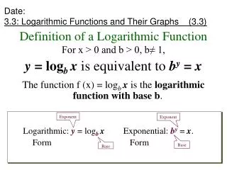
(A) Graph of Logarithmic Functions • Graph the exponential function f(x) = 2x and then graph the inverse y = f-1(x) which is x = 2y. This inverse is called a logarithm and is written as y = log2(x) • After seeing the graph, we can analyze the features of the graph of the logarithmic function
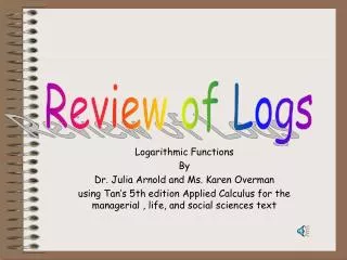
Exponential Fcns: x y -5.00000 0.03125 -4.00000 0.06250 -3.00000 0.12500 -2.00000 0.25000 -1.00000 0.50000 0.00000 1.00000 1.00000 2.00000 2.00000 4.00000 3.00000 8.00000 4.00000 16.00000 5.00000 32.00000 6.00000 64.00000 7.00000 128.00000 Logarithmic Fcns: x y 0.03125 -5.00000 0.06250 -4.00000 0.12500 -3.00000 0.25000 -2.00000 0.50000 -1.00000 1.00000 0.00000 2.00000 1.00000 4.00000 2.00000 8.00000 3.00000 16.00000 4.00000 32.00000 5.00000 64.00000 6.00000 128.00000 7.00000 (A) Tables of Values for Exponentials and Logarithmic Functions
(B) Analyzing Graphs of Logarithms • So we can now do a complete graphic analysis of this graph • (i) no y-intercept and the x-intercept is 1 • (ii) the y axis is an asymptote • (iii) range {yER} • (iv) domain {x > 0} • (v) it increases over its domain • (vi) it is concave down over its domain • (vi) it has no max/min or turning points
(C) Graphs of Transformed Logarithmic Functions • As will be seen in the next exercises, the graph maintains the same “shape” or characteristics when transformed • Depending on the transformations, the various key features (domain, range, intercepts, asymptotes) will change
(D) Investigating the Logarithmic Function f(x) = alogB[b(x + c)] + d • Go to this link Logarithmic Functions from AnalyzeMath and work through the tutorial on transformed logarithmic functions • Consider how y = logB(x) changes i.e. the domain, range, asymptotes, increasing/decreasing nature of the function, shifting and reflecting
(E) Graphing the Logarithmic Function Without Graphing Technology • Recall the key features of the logarithmic function, y = log(x): • domain {x E R |x > 0} • Range is y E R • Vertical asymptotes y axis (or the line x=0) • X-intercept (1,0) • The function increases over its entire domain
(E) Graphing Log Functions • Without using graphing technology, graph the following functions (it may help to recall your knowledge of function transformations) • (1) f(x) = log2(x + 2) • (2) f(x) = -3log2(x - 4) • (3) f(x) = log5(4x – 4) + 5 • Examples and discussions on how to make these graphs is found at the following website: • Graphs of Logarithmic Functions from AnalyzeMath
(F) Homework • Nelson Text, page 118, Q9, 10, 12, 15, 21