Forecasting Correlation and Covariance with a Range-Based Dynamic Conditional Correlation Model

1. Forecasting Correlation and Covariance with a Range-Based Dynamic Conditional Correlation Model Ray Y Chou Institute of Economics Academia Sinica Nathan Liu National Chiao Tung University Chun-Chou Wu Chung Yuan University

2. Outline • Introduction • Dynamic Conditional Correlation (DCC) Model • Methodology • Data Analysis • Empirical Analysis • Conclusion

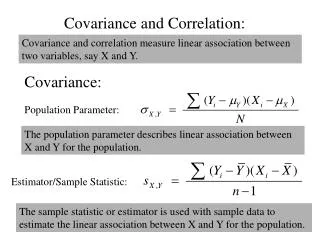
3. Introduction • It is of primary importance in the practice of portfolio management, asset allocation and risk management to have an accurate estimate of the covariance matrices for asset prices. • The univariate ARCH/GARCH family of models provides effective tools to estimate the volatilities of individual asset prices, see Bollerslev, Chou and Kroner (1992), Engle (2004). • It is an active research issue in estimating the covariance or correlation matrices of multiple, including VECH model of Bollerslev, Engle and Wooldridge (1988), BEKKmodel of Engle and Kroner (1995) and the constant correlation model of Bollerslev (1990) among others.

4. Introduction (Cont.) • The constant correlation model istoo restrictive as it precludes the dynamic structure of covariance to be completely determined by the individual volatilities. • The VECH and the BEKK models are more flexible in allowing time-varying correlations. Nevertheless the computational difficulty of the estimation of the model parameters has limited the application of these models to only small number of assets. • Engle and Sheppard (2001), Engle (2002a) and Engle, Cappiello and Sheppard (2003) provide a solution to this problem by using a model entitled the Dynamic Conditional Correlation Multivariate GARCH (henceforth DCC).

5. Introduction (Cont.) • Other estimation methods of time-varying correlation are proposed by Tsay (2002) and by Tse and Tsui (2002). • there is a growing awareness of the fact that the high/low range data of asset prices can provide sharper estimates and forecasts than the return data based on close-to-close prices. Studies of suppoting evidences include Parkinson (1980), Garman and Klass (1980), Wiggins (1991), Rogers and Satchell (1991), Kunitomo (1992), and more recently Gallant, Hsu and Tauchen (1999), Yang and Zhang (2000), Alizadeh, Brandt and Diebold (2001), Brandt and Jones (2002), Chou, Liu and Wu (2003) and Chou (2005a, 2005b).

6. Traditional Conditional Covariance and Correlation Moving Average with a 100-week window, MA(100) Conditional Covariance/Correlation

7. Conditional Covariance/Correlation • Exponentially-Weighted Moving Average (EWMA) model where the weights decrease exponentially As to the coefficient is usually called the exponential smoother in this model by RiskMetrics.

8. Dynamic Conditional Correlation model • The multivariate GARCH model proposed assumes that returns from k assets are conditionally multivariate normal with zero expected value and covariance matrix Ht. where Dtis the kxk diagonal matrix of time varying standard deviations from univariate volatility models with the square root ofon thediagonal, and is the time varying correlation matrix.

9. Dynamic Conditional Correlation model (Cont.) • It is important to recognize that although the dynamic of theDt matrix has usually been structured as a standard univariate GARCH, it can take many other forms. • The standardized series is , hence are the residuals standardized by their conditional standard deviation. • A general dynamic correlation structure proposed by Engle (2000a) is:

10. Dynamic Conditional Correlation model (Cont.) • where Sis the unconditional covariance of the standardized residuals. where iis a vector of ones and o is the Hadamard product of two identically sized matrices which is computed simply by element by element multiplication. It’s shown that if A , B, and(ii’-A-B)are positive semi-definite, then Q will be positive semi-definite. • The typical element of Rtwill be of the form . • Engle and Sheppard (2001) show the necessary conditions for Rt to be positive definite and hence a correlation matrix with a real, symmetric positive semi-definite matrix, with ones on the diagonal.

11. Dynamic Conditional Correlation model (Cont.) • The loglikelihood of this estimator can be written: • Let the parameters in Dt be denoted and the additional parameters in Rt be denoted .

12. Dynamic Conditional Correlation model (Cont.) • The log likelihood can written as the sum of a volatility part and a correlation part. The volatility term is: and the correlation component is:

13. Dynamic Conditional Correlation model (Cont.) • The volatility part of the likelihood is the sum of individual GARCH likelihood if Dt is determined by a GARCH specification which can be jointly maximized by separately maximizing each term. If Dt is determined by a CARR specification, where is the conditional standard deviation as computed from a scaled expected range from the CARR model.

14. Dynamic Conditional Correlation model (Cont.) • The second part of the likelihood will be used to estimate the correlation parameters. As the squared residuals are not dependent on these parameters, they will not enter the first order conditions and can be ignored. • The two step approach to maximizing the likelihood is to find and then take this value as given in the second stage,

15. Methodology • For bivariate cases, we use the following GARCH and CARR model to perform the first step procedure in estimating the volatility parameters: GARCH（return-based conditional volatility model） ,k=1,2 • CARR（range-based conditional volatility model） ,k=1,2 ,where ,

16. Methodology (Cont.) • In estimating the correlation parameters, we also allow two specifications of the dynamic structures in the correlation matrix. • MR_DCC (mean-reverting)

17. Methodology (Cont.) • I_DCC (integrated)

18. Methodology (Cont.) • The estimated conditional correlation coefficients are • Like volatilities, the correlation and covariance matrices are also unobservable. We use daily data to construct weekly realized covariance/correlation observations. • The purpose of this is to use these “measured covariance/ correlation” denoted MCOV/MCORR respectively as benchmarks in determining the relative performance of the return-based DCC model and the range-based DCC models.

19. Methodology (Cont.) • We perform the Mincer-Zarnowitz regressions for the in-sample comparison： where

20. Methodology (Cont.) • Following Engle and Sheppard (2001), the out-of-sample conditional correlations MR_DCC are computed. For T+h, with , the correlation is

21. Data Analysis • The data employed in this study comparises 835 weekly observations on the S&P 500 Composite (henceforth S&P 500), NASDAQ stock market index and bond yield for 10 years time to maturities spanning the period 4 January 1988 to 2 January 2004. Two variant DCC structures to estimate the model’s significance are investigated. • Let MCORRt and MCOVt represent the realized multi-correlation coefficients and multi-covariances, respectively. The MCORRt is defined as: where symbol the tradable days during the t week

22. Data Analysis (Cont.) • is called the correlation coefficient at the i trading day of the week based on two indices that we have selected. We can use the daily returns data and fit them into the MR_DCC model, so that the can be computed. The multi-covariances (MCOVt) can be expressed as • Where represents the daily returns of k index at the i trading day during the t week.

23. Summary Statistics

24. Return- Versus Range-based DCC Models In-sample MCORR Forecasting

25. Correlation fitting (S&P500 and Bond)

26. The Time-Varying Correlation

27. The Time-Varying Correlation

28. Return- Versus Range-based DCC Models In-sample MCOV Forecasting

29. Return- versus Range-based DCC Models Out-of-Sample MCORR Forecasting

30. Return- versus Range-based DCC Models Out-of-Sample MCOV Forecasting

31. Conclusion • A new estimator of the time-varying correlation/covariance matrices is proposed utilizing the range data by combining the CARR model of Chou (2005a) and the framework of Engle (2002)’s DCC model. • We find consistent results that the range-based DCC model outperforms the return-based models in estimating and forecasting covariance and correlation matrices, both in-sample and out-of-sample. • It can be applied to larger systems in a manner similar to the application of the return-based DCC model structures that is demonstrated in Engle and Sheppard (2001). • Future research will be useful in adopting more diagnostic statistics or tests based on value at risk calculations as is proposed by Engle and Manganelli (1999).