Download
1 / 31
310 likes | 414 Views
6dB Better than CW. Weak Signal Modes on the Microwave Bands Andy Talbot G4JNT/G8IMR. Traditional CW. Is the weak signal mode used when all else (especially SSB !) fails Limited by Noise – Proportional the bandwidth Operators ability to decode it Often need to repeat messages

E N D
6dB Better than CW Weak Signal Modes on the Microwave Bands Andy Talbot G4JNT/G8IMR
Traditional CW Is the weak signal mode used when all else (especially SSB !) fails Limited by Noise – Proportional the bandwidth Operators ability to decode it Often need to repeat messages Talkback / handshaking Alphabet prone to errors if message is broken J (--- --- ---) = E E M (- - -- --)
A few Values • Ear / Brain combination is surprisingly good at detecting tones buried in noise • SSB voice needs ~ 3kHz for full readability • We detect it as if the bandwidth were only a few tens of Hz • And especially tones at the right frequency, in something like 20 – 100Hz noise bandwidth • This often gives a false impression how good a signal really is.
Some Audio Generated by Maths! Sampling Rate 8000 Hz --- 16 Bit sampling, noise RMS = -10dB S/N Ref BW 2500 Hz -5dB = 32767 / SQRT(10) = 10361 Audio BW 100 Hz -19dB 99% probability of no clipping Signal/Noise Source File Amplitude Dest File Noise 2.5kHz 100Hz dB wrt FSD dB FSD Norm. Audio CWMSGM20 -20 ..\dsp\weakcw01.wav -10 -5 9 CWMSGM25 -25 ..\dsp\weakcw02.wav -10 -10 4 CWMSGM30 -30 ..\dsp\weakcw03.wav -10 -15 -1 CWMSGM35 -35 ..\dsp\weakcw04.wav -10 -20 -6CW Limit ? CWMSGM40 -40 ..\dsp\weakcw05.wav -10 -25 -11
The Limit for CW • At best, around 10dB S/N in 30Hz for easy copy CW. No repeats • Several dB lower for detecting • Assume 18WPM at this level. • A Word has 5 chars, 4.5 bits / char (plain text) = 6 or 7 Bits /second equiv data rate • Repeat the message, gives ~ 2 -3 Bits/s • This is manual Forward Error Correction
Compare simple data modes • RTTY 30 Bits/s (for 50 baud) • Needs >15dB S/N in 100Hz (around the two tones) • Very inefficient • PSK31 >10dB S/N in 31Hz • About the same as CW with a good operator • Both of these are error prone, so repeats are needed • Reduces overall data rate
And what about Microwave Bands? • Rain Scatter • Spreads the signal over 100 – 300Hz • CW survives this quite well, (and RS is often strong) • DFCW with spectral display works reasonably well • Scattering / breakup / troposcatter / multipath • Kills CW • Kills most other data modes
Can we go Narrower • Yes - Lower BW , less noise, increases S/N • But the message takes proportionately longer to send • Spreading could be a problem • Need machine assistance • QRSS, Visual CW, DFCW, Hell • ‘About the same signalling efficiency as CW’
Visual CW / DFCW / DFCWi Advantages for very slow data in narrow band – about same as aural CW when scaled for speed/BWidth.
Can We Do Better • Yes – but there is a theoretical limit • Shannon suggests two routes • Improve the signalling efficiency with better modulation (move left) • Not much scope with modern modulations • Increase the bandwidth (move up) • This appears counter-intuitive BUT---------- • The maths sez so
The Shannon CurveWas derived from basic Physics / Maths / Info theory and is NOT an experimental result. It is a TARGET. • Horizontal – Normalised Signal/Noise, energy / bit • Move left, Lower Tx power, or increase noise • Vertical – Spectral Efficiency, Bits/s/Hz. • Move up, increase bandwidth for same capacity • Red – 2 … 32 PSK/QAM • Blue – 2 … 64 MFSK • Purple - Heavily coded deep space • Red Line – “10dB from Shannon “ Can’t go here http://marconig.wordpress.com/2007/07/03/the-shannon-capacity-curve/
Bandwidth Expansion • Commercially / military use spread spectrum • WLAN, Bluetooth, Wi-Fi. • All improve signalling efficiency by spreading the signal over a wide bandwidth to counter interference / multipath • Not too easy on the Am. Bands as we nearly always want to keep within the 3kHz SSB bandwidth
Another Way • Heavy Error Correction • Often not thought-of as a bandwidth spreading • We already see it in normal operation – • Repeat the information many times • Slowing the data rate and keeping the same modulation format is equivalent to widening the bandwidth • It’s the ratio of Data Rate / Bandwidth that matters
Source Coding • First Get rid of redundant information (WSJT Style) • Compress callsigns using their known structure • Char-Char-Number-Letter-Letter-Letter • Letter = A-Z or [space]. Char = Letter or 0-9 (but note the 2nd Char cannot be a [space]) • Compresses to 37*36*10*27*27*27 = 262Meg • Which can be represented by 28 Bits • (RTTY needs at least 35 bits, could be more depending on letter/figure shift) • Locator (4 digit) 18*18*10*10 = 32400 (15 Bits) 6 Digit Loc 25 bits
Further Source Coding • Assume 4 Million Radio Ams in the world (we wish!) • Use a codebook to store the callsign of everyone, then just transmit the reference number • Only needs 22 bits • This is contentious lets not go there ! • Reports and acknowledgements need only a few bits in reality • But this also sparks controversey • With the natural redundancy removed, any random data message begins to look valid • Acknowledged ‘problem’ with source coding
An Aside…. • Morse is a classic example of source coding • Most common letters use less data bits than less popular ones • Same problem of one symbol being corrupted to another • eg. T = E E • Bleeps from continuity tester can spell messages
Modulation • On-Off, or Amplitude Shift Keying is not good. • It must waste 3dB • PSK is theoretically the best (multiplication by 1 or -1) • Maintains high duty/cycle • Coherency needs frequency / phase lock • Which can be destroyed by propagation anomalies • Non-linear processing for recovery throws away many of the advantages of coherent reception • Unless bandwidth is unimportant, needs linear transmitters • Which leaves good old fashioned, well established FSK
Multi FSK • Use several Tones • Extend these over more than the anticipated spread • 10’s of Hz for V/UHF. • 100’s of Hz for microwave • All well within the 3kHz SSB bandwidth. • 4 tones give 2 bits per symbol • F0 = ’00’, F1 = ’01’, F2 = ’11’, F3 = ’10’ WSPR / JT4 • 64 tones 6 bits per symbol • F0 = ‘000000’, F7 = ‘000111’, F26 = ‘011010’, F63 = ‘111111’ JT65 • We’ve increased our data rate at the expense of decodng complexity – that’s no problem these days
Error Correction • Now make good use of our increased capacity / data rate • Could just repeat the message several times and compare each, looking for errors in each bit. • Three repeats allows error correction • Two repeats allows detection – may be enough if talkback allows a repeat request • Interleave the repeats to counter burst errors • But we can do a lot better • and its very mathematical
Error Correction Techniques • Hamming Distance • Add enough extra parity bits so the new alphabet has a certain number of bits different between each block. Then compare each received one and look for the most probable. • Example is 4 bits with 3 more parity • Allows 1 error in a total of 7 to be corrrected • 2 errors can be detected • Simple schemes are decoded using lookup tables • Block coding • More efficient longer-word schemes are in widespread use • Reed-Solomon, BCH • But the maths processing is NOT NICE • Galois Fields, Dividing Polynomials
Error Correction Techniques continued • Convolutional Coding • Continuously spread each source over several bits of the output. Adding more for correction – eg x2 or x3 • Continuously look for what was most likely to have been sent in order to generate what has actually been received. • Soft decision decoding looks at probability a received symbol is good, bad or indifferent • The Viterbi decoding algorithm • Searches back though received symbols in a trellis, looking for the most likely data that could have generated it • Processor intensive, adds a delay.
Another Aside A few state-of-the art codes • Taken from • http://marconig.wordpress.com/2007/07/03/the-shannon-capacity-curve/ • These are for BPSK with the coding used with several deep space (interplanetary) spacecraft: • r=1/2 k=7 convolutional: Eb/No 4.5 dB, eff 0.5 bps/Hz • Voyager (RS+r=1/2,k=7): Eb/No 2.4 dB, eff 0.437 bps/Hz • Cassini (RS+r=1/6 k=15): Eb/No 0.6 dB, eff 0.146 bps/Hz • CCSDS r=1/6 turbo large block: Eb/No 0.0 dB 0.167 bps/Hz • Not much scope for further improvement
Timing and Frequency Errors • Need knowledge of frequency / tuning error and timing • Use UTC based protocol to limit search requirements • Identify Start of message timing • To be able to identify the right symbols • Can’t afford to spend a lot of time searching • Typical few seconds for PC clock errors, bit more for EME delays • Frequencyget within a tone bandwidth for MFSK schemes. • Send synchronisation Sequence • Unique pattern to search for that won’t appear anywhere in the message. Can give frequency and time.
WSJT Examples • JT65 • 72 source Bits - 2 compressed callsigns + one 4-digit Locator OR 13 chars of plain text. • Block coding (Reed Solomon) expanded to 126 symbols of 64 tones (6 bits / symbol) ,and one more for sync , Pseudo Random interspersed. • Effectively expands a 72 bit message to an effective 441 bits • Big Sync overhead – 50% of the message time • Three tone spacings, 2.7, 5.4 and 10.8Hz
JT4 a-g and WSPR • Both similar coding schemes • Four tones carrying two bits per symbol, • One bit is sync sent as a pseudo-random code • The other is a data bit • JT4 same message as JT65, • 72 bits expanded to 207 in a convolutional encoder • Sent in 48 seconds at 4.375 symbols/s • Tone spacing user selected from 4.4 to 315Hz • WSPR Different Message, new data structure • 50 bits expanded to 162 in a convolutional encoder • Sent in 110 seconds at 1.46 symbols / second • Tone spacing 1.46Hz
Using WSJT • Setup Box • Callsign, Locator, Com Port for Tx control • Make Sure sampling rate calibration is OK • (Only done once per PC – unless using .WAV files). Look at Self Check value. Enter into Setup, Options • Set The right Mode (easily forgotton!) • Set PC Clock • Dsec Box for fine tuning – aim for less than a second or two error from UTC • Adjust Audio Levels • Need Rx or Monitor to be running
Run WSJT........... Load in .WAV files from GB3SCX and GB3SCS Set Rate in to 1.0068 (Saved on a different machine) Replay .WAV files and use mic to loop round Set Options Rate-in back to to 0.9797 - check value. (Although they were recorded on another machine at 11100Hz, check exact value!) Use Monitor mode and start VLC replay 2 seconds early
Where to hear WSJT Signals • Off the Moon , JT65A, B, C • GB3SCX 10368.905MHz JT4G • GB3SCS 2320.905MHz JT4G • Tune so USB carrier is 800Hz below • GB3VHF 144.43MHz JT65B • Tune 1500Hz low, USB carrier 144.4285MHz • GB3RAL 40.05/50.05/60.05/70.05 JT65B • Tune USB carrier Xx.0485MHz • HF Bands JT65A, JT4A+, WSPR