Test rooms: Instructor Sections Room Dr. Hale F, H 104 Physics Dr. Kurter B, N 125 BCH

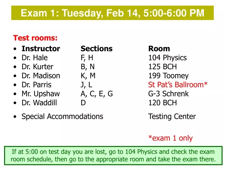
Exam 1: Tuesday, Feb 14, 5:00-6:00 PM Test rooms: • Instructor Sections Room • Dr. Hale F, H 104 Physics • Dr. Kurter B, N 125 BCH • Dr. Madison K, M 199 Toomey • Dr. Parris J, L St Pat’s Ballroom* • Mr. Upshaw A, C, E, G G-3 Schrenk • Dr. Waddill D 120 BCH • Special Accommodations Testing Center *exam 1 only If at 5:00 on test day you are lost, go to 104 Physics and check the exam room schedule, then go to the appropriate room and take the exam there.

Testing center reservations • I have made reservations for all students who have given me their accommodation letter • You should have received a reservation email from the testing center • You must make your own appointment in addition to my reservation (unless you have already done so) • If you believe you should be in the testing center but have not received a reservation email, let me know now!

Today’s agenda: Electric potential of a charge distribution. You must be able to calculate the electric potential for a charge distribution. Equipotentials. You must be able to sketch and interpret equipotential plots. Potential gradient. You must be able to calculate the electric field if you are given the electric potential. Potentials and fields near conductors. You must be able to use what you have learned about electric fields, Gauss’ law, and electric potential to understand and apply several useful facts about conductors in electrostatic equilibrium.

Electric potential V of charge distributions • last lecture: potentials of point charges • now: potentials of extended charged objects • (line charges, sheet charges, spheres, cylinders, etc) • Two strategies: • decompose distribution into charge elements, integrate their contributions to V • first find the electric field of the distribution (for example via Gauss’ law), then integrate

Example 1: electric potential between two parallel charged plates. • plates carry surface charge density  • plates separated by distance d • plates are large compared to d , perpendicular to plates E _ d +

y x E z dl V is higher at the positive plate V0 V1 d |V|=Ed The (in)famous “Mr. Ed equation!*” holds for constant field only *2004, Prof. R. E. Olson.

Example 2:A thin rod of length L located along the x-axis has a total charge Q uniformly distributed along the rod. Find the electric potential at a point P along the y-axis a distance d from the origin. Follow line charge recipe 1. Decompose line charge 2. Potential due to charge element dq=dx y * =Q/L P r d Q dq x dx x L *What are we assuming when we use this equation?

3. Integrate over all charge elements Use integral: y P r d Q dq x dx x L Include the sign of Q to get the correct sign for V. note: ln(a) – ln(b) = ln(a/b) What is the direction of V?

Example 3:Find the electric potential due to a uniformly charged ring of radius R and total charge Q at a point P on the axis of the ring. dq Every dq of charge on the ring is the same distance from the point P. r R P x x Q

Could you use this expression for V to calculate E? Would you get the same result as I got in Lecture 3? dq r R P x x Q Homework hint: you must derive this equation in tomorrow’s homework!

Example 4:Find the electric potential at the center of a uniformly charged ring of radius R and total charge Q. dq R Every dq of charge on the ring is the same distance from the point P. P Q

Example 4: A disc of radius R has a uniform charge per unit area  and total charge Q. Calculate V at a point P along the central axis of the disc at a distance x from its center. we already know V for a ring • decompose disk into rings • area of ring of radius r′ and thickness dr’ is dA=2r′dr’ • charge of ring is dq= dA = (2r′dr′) with =Q/R2 dq r′ P x x R Q each ring is a distance from point P

dq r′ P x x R Q This is the (infinitesimal) potential for an (infinitesimal) ring of radius r′. On the next slide, just for kicks I’ll replace k by 1/40.

dq r′ P x x R Q

Could you use this expression for V to calculate E? Would you get the same result as I got in Lecture 3? dq r′ P x x R Q

Example 5: calculate the potential at a point outside a very long insulating cylinder of radius R and positive uniform linear charge density . Which strategy to use? • decomposition into charge elements and • leads to complicated triple (volume) integral NO! • calculate first, then use • we already derived using Gauss’ law YES! To be worked at the blackboard in lecture…

r r=a >0  E dr r=R R Start with and to calculate

r r=a >0  E dr r=R R

If we let a be an arbitrary distance r, then If we take V=0 at r=R, then

Things to note: If we tried to use V=0 at r= then (V is infinite at any finite r). That’s another reason why we can’t start with V is zero at the surface of the cylinder and decreases as you go further out. This makes sense! V decreases as you move away from positive charges.

Things to note: For >0 and r>R, Vr – VR <0. Our text’s convention is Vab = Va – Vb. This is explained on page 759. Thus VrR = Vr – VR is the potential difference between points r and R and for r>R, VrR < 0. In Physics 1135, Vba = Va – Vb. I like the Physics 1135 notation because it clearly shows where you start and end. But Vab has mathematical advantages which we will see in Chapter 24.

Equipotentials Equipotentials are contour maps of the electric potential. http://www.omnimap.com/catalog/digital/topo.htm

Equipotential lines: • lines of constant electric potential V • visualization tool complementing electric field lines Electric field is perpendicular to equipotential lines. Why? Otherwise work would be required to move a charge along an equipotential surface, and it would not be equipotential. In static case (charges not moving), surface of conductor is an equipotential surface. Why? Otherwise charge would flow and it wouldn’t be a static case.

Here are electric field and equipotential lines for a dipole. Equipotential lines are shown in red.

Potential Gradient (Determining Electric Field from Potential) Electric field vector points from + to -, this means from higher to lower potentials. Remember: Inverse operation: E E is perpendicular to the equipotentials

For spherically symmetric charge distribution: In one dimension: In three dimensions:

Example (from a Fall 2006 exam problem): In a region of space, the electric potential is V(x,y,z) = Axy2 + Bx2 + Cx, where A = 50 V/m3, B = 100 V/m2, and C = -400 V/m are constants. Find the electric field at the origin

Potentials and Fields Near Conductors When there is a net flow of charge inside a conductor, the physics is generally complex. When there is no net flow of charge, or no flow at all (the electrostatic case), then a number of conclusions can be reached using Gauss’ Law and the concepts of electric fields and potentials…

Eletrostatics of conductors Electric field inside a conductor is zero. Any net charge on the conductor lies on the outer surface. Potential on the surface of a conductor, and everywhere inside, is the same. Electric field just outside a conductor must be perpendicular to the surface. Equipotential surfaces just outside the conductor must be parallel to the conductor’s surface.

Test rooms: Instructor Sections Room Dr. Hale F, H 104 Physics Dr. Kurter B, N 125 BCH