Download
1 / 18
180 likes | 241 Views
h elicity distribution and measurement of N spin. in general, g 1 (x B ,Q 2 ) : dependence on Q 2 (= scaling violations) calculable in perturbative QCD interest in g 1 ( x B ,Q 2 ) is due to its 1 o Mellin moment

E N D
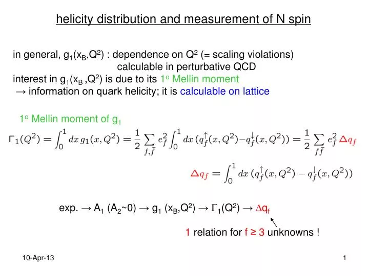
helicity distribution and measurement of N spin in general, g1(xB,Q2) : dependence on Q2 (= scaling violations) calculable in perturbative QCD interest in g1(xB,Q2) is due to its 1oMellin moment → information on quark helicity; it is calculable on lattice 1oMellin moment of g1 exp. → A1 (A2~0) → g1 (xB,Q2) → 1(Q2) →qf 1 relation for f≥ 3 unknowns !
(cont’ed) in QPM for proton : QPM : wave function of q in P↑“induced” by SUf(3) ⊗ SU(2) → 1p = 5/18 ~0.28 = 1 3 unknowns → info from axial current Aa~5Ta in semi-leptonic decays (ex. decay) in baryonic octet Result: from a fit to semi-leptonic decays → F= 0.47 ± 0.004 ; D=0.81± 0.003 Ellis-Jaffe sum rule(’73) (hp.= perfect symmetry SUf (3) + s=0 ) complicated corrections
Experiment EMC (CERN, ’87) ↑p↑→p at Q2 = 10.7 GeV2 R = L/T from unpolarized cross section confirmed also from: SMC (Cern), E142 and E143 (SLAC)
Spin crisis F + D + 1p (Q2) →Σand u, d, s Q2 = 10.7 GeV2 = 0.13 ± 0.19 u = 0.78 ± 0.10 d = 0.50 ± 0.10 s = -0.20 ± 0.11 negative sea polarization Q2 = 3 GeV2 = 0.27 ± 0.04
(cont’ed) QPM Ellis – Jaffe sum rule exp. SUf (3) + s=0 1p = 0.17 ± 0.01 = 0.60 ± 0.12 Q2 = 10.7 GeV2 1p = 0.126 ± 0.010 ± 0.015 = 0.13 ± 0.19 Q2 = 3 GeV2 = 0.27 ± 0.04 1p~ 0.28 = 1 discrepancy > 2 Violation of SUf (3) ? extrapolating g1(x) for x → 0 ? none of them quantitatively explains observeddiscrepancy axial anomaly → gluon contribution ?
from weakcouplings in decay of N polarizedBjorken sum rule axial pQCD corrections vector QPM: wave function of q in P according to SUf(3) ⊗SU(2) exp. 1.267 ± 0.004 Sum rule :
inclusivee+e- annihilations q = k+k’ time-like q2≡Q2 = s≥ 0 k k’ average on initial polarizations
(cont’ed) QPM picture only Nc ways of creating a pair by conserving color in vertex no hadrons in initial and final states in QPM ≡ elementary Q2 = s such that only are produced Q2 (e+e-→X) scales !
hence evidence of Nc test of gauge structures SUc (3) and SUf (3) below c threshold R = 3 (4/9 + 2/9) = 2 around threshold resonances J/, ’ above c threshold R = 2 + 3 4/9 = 3+1/3 ….. seealso Wu, Phys.Rep. C107 59 (84)
inclusivee+e- annihilations (factorization) theorem : total cross section is finite in the limit of massless particles, i.e. it is free from “infrared” (IR) divergences (Sterman, ’76, ’78) [generalization of theorem KLN (Kinoshita-Lee-Nauenberg)] QPM pQCD corrections
inclusivee+e- PX J(0) J(0) theorem: dominant contribution in Bjorken limit comes from short distances → 0 (on the light-cone) but product of operators in the same space-time point is not always well defined in field theory !
(cont’ed) Example: free neutral scalar field (x) ; free propagator (x-y) K1 modified Bessel funct. of 2nd kind Example: interacting neutral scalar field (x) depends only on p2=m2 → it is a constant N
Operator Product Expansion (Wilson, ’69 first hypothesis; Zimmermann, ’73 proof in perturbation theory; Collins, ’84 diagrammatic proof) (operational) definition of composite operator: • local operators Ôi are regular for every i=0,1,2… • divergence for x → y is reabsorbed in coefficients Ci • terms are ordered by decreasing singularity in Ci , i=0,1,2… • usually Ô0 = I , but explicit expression of the expansion must be • separately determined for each different process • OPE is also an operational definition because it can be used • to define a regular composite operator. • Example : theory 4 ; the operator (x)2 can be defined as
the Wick theorem scalar field “normal” order : : = move a† to left, a to right → annihilate on |0> “time” order T = order fields by increasing times towards left Step 1 Step 2 t2<t1 analogously for t2>t1 hence recursive generalization
analogously non interacting fermion fields general formula of Wick theorem: Pij = (-1)m m= n0 of permutations to reset indices in natural order 1, … ,i-1,i, … ,j-1,j, ... ,n
application to inclusive e+e- and DIS W ⇒ J() J(0) with Je.m. current of quark normal product : : useful to define a composite operator for → 0 ⇒ study T[J() J(0)] per → 0 with Wick theorem divergent for → 0 ⇒ OPE
singularities of free fermion propagator light-cone singularity degree of singularity proportional to powers of q in Fourier transform highest singularity in OPE coefficients dominant contribution to J in W
(cont’ed) mostsingular term in T [J() J(0)] lesssingular term in T [J() J(0)] regular bilocal operator