Download
1 / 18
270 likes | 562 Views
Optimization with Constraints. Standard formulation Why are constraints a problem? Canyons in design space Equality constraints are particularly bad!. Derivative-based optimizers. All are predicated on the assumption that function evaluations are expensive and gradients can be calculated.

E N D
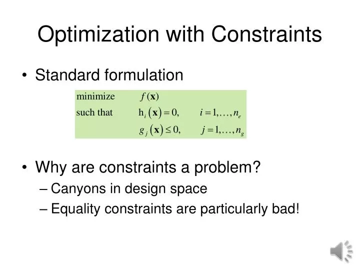
Optimization with Constraints • Standard formulation • Why are constraints a problem? • Canyons in design space • Equality constraints are particularly bad!
Derivative-based optimizers • All are predicated on the assumption that function evaluations are expensive and gradients can be calculated. • Similar to a person put at night on a hill and directed to find the lowest point in an adjacent valley using a flashlight with limited battery • Basic strategy: • Flash light to get derivative and select direction. • Go straight in that direction until you start going up or hit constraint. • Repeat until converged. • Steepest descent does not work well. For unconstrained problems use quasi-Newton methods.
Gradient projection and reduced gradient methods • Find good direction tangent to active constraints • Move a distance and then restore to constraint boundaries • How do we decide when to stop and restore?
The Feasible Directions method • Compromise constraint avoidance and objective reduction
Penalty function methods • Quadratic penalty function • Gradual rise of penalty parameter leads to sequence of unconstrained minimization technique (SUMT). Why is it important?
Contours for r=1000 . For non-derivative methods can avoid this by having penalty proportional to absolute value of violation instead of its square!
Multiplier methods • By adding the Lagrange multipliers to penalty term can avoid ill-conditioning associated with high penalty
Can estimate Lagrange multipliers • Stationarity • Without penalty • So: • Iterate See example in textbook
5.9: Projected Lagrangian methods • Sequential quadratic programming • Find direction by solving • Find alpha by minimizing
Matlab function fmincon FMINCON attempts to solve problems of the form: min F(X) subject to: A*X <= B, Aeq*X = Beq (linear cons) X C(X) <= 0, Ceq(X) = 0 (nonlinear cons) LB <= X <= UB X=FMINCON(FUN,X0,A,B,Aeq,Beq,LB,UB,NONLCON) subjects the minimization to the constraints defined in NONLCON. The function NONLCON accepts X and returns the vectors C and Ceq, representing the nonlinear inequalities and equalities respectively. (Set LB=[] and/or UB=[] if no bounds exist.) [X,FVAL]=FMINCON(FUN,X0,...) returns the value of the objective function FUN at the solution X. What does the order of arguments in fmincon tell you about the expectations of Matlab on the most common problems to be solved?
Useful additional information [X,FVAL,EXITFLAG] = fmincon(FUN,X0,...) returns an EXITFLAG that describes the exit condition of fmincon. Possible values of EXITFLAG 1 First order optimality conditions satisfied. 0 Too many function evaluations or iterations. -1 Stopped by output/plot function. -2 No feasible point found. [X,FVAL,EXITFLAG,OUTPUT,LAMBDA] = fmincon(FUN,X0,...) returns Lagrange multipliers at the solution X: LAMBDA.lower for LB, LAMBDA.upper for UB, LAMBDA.ineqlin is for the linear inequalities, LAMBDA.eqlin is for the linear equalities, LAMBDA.ineqnonlin is for the nonlinear inequalities, and LAMBDA.eqnonlin is for the nonlinear equalities.
Ring Example Quadratic function and constraint function f=quad2(x) Global a f=x(1)^2+a*x(2)^2; function [c,ceq]=ring(x) global riro c(1)=ri^2-x(1)^2-x(2)^2; c(2)=x(1)^2+x(2)^2-ro^2; ceq=[]; x0=[1,10]; a=10;ri=10.; ro=20; [x,fval]=fmincon(@quad2,x0,[],[],[],[],[],[],@ring) x =10.0000 -0.0000 fval =100.0000
Making it harder for fmincon • >> a=1.1; • [x,fval]=fmincon(@quad2,x0,[],[],[],[],[],[],@ring) • Warning: Trust-region-reflective method does not currently solve this type of problem, • using active-set (line search) instead. • > In fmincon at 437 • Maximum number of function evaluations exceeded; • increase OPTIONS.MaxFunEvals. • x =4.6355 8.9430 fval =109.4628
Restart sometimes helps >>x0=x x0 = 4.6355 8.9430 >> [x,fval]=fmincon(@quad2,x0,[],[],[],[],[],[],@ring) • x =10.0000 0.0000 • fval =100.0000 • Why restarting a solution is often more effective than having a large number of iterations in the original search?