Download
1 / 123
1.23k likes | 1.24k Views
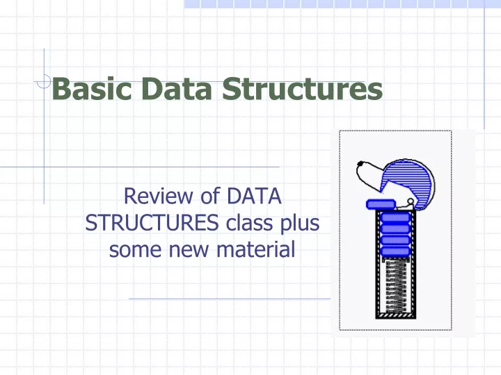
Basic Data Structures. Review of DATA STRUCTURES class plus some new material. Stacks. An abstract data type (ADT) is an abstraction of a data structure An ADT specifies: Data stored Operations on the data Error conditions associated with operations.

E N D
Basic Data Structures Review of DATA STRUCTURES class plus some new material
An abstract data type (ADT) is an abstraction of a data structure An ADT specifies: Data stored Operations on the data Error conditions associated with operations Example: ADT modeling a simple stock trading system The data stored are buy/sell orders The operations supported are order buy(stock, shares, price) order sell(stock, shares, price) void cancel(order) Error conditions: Buy/sell a nonexistent stock Cancel a nonexistent order Abstract Data Types (ADTs)
The Stack ADT stores arbitrary objects Insertions and deletions follow the last-in first-out scheme Think of a spring-loaded plate dispenser Main stack operations: push(object): inserts an element object pop(): removes and returns the last inserted element Auxiliary stack operations: object top(): returns the last inserted element without removing it integer size(): returns the number of elements stored boolean isEmpty(): indicates whether no elements are stored The Stack ADT
Attempting the execution of an operation of ADT may sometimes cause an error condition, called an exception Exceptions are said to be “thrown” by an operation that cannot be executed In the Stack ADT, operations pop and top cannot be performed if the stack is empty Attempting the execution of pop or top on an empty stack throws an EmptyStackException Exceptions
Applications of Stacks • Direct applications • Page-visited history in a Web browser • Undo sequence in a text editor • Chain of method calls in the Java Virtual Machine • Indirect applications • Auxiliary data structure for algorithms • Component of other data structures
Method Stack in the JVM main() { int i = 5; foo(i); } foo(int j) { int k; k = j+1; bar(k); } bar(int m) { … } • The Java Virtual Machine (JVM) keeps track of the chain of active methods with a stack • When a method is called, the JVM pushes on the stack a frame containing • Local variables and return value • Program counter, keeping track of the statement being executed • When a method ends, its frame is popped from the stack and control is passed to the method on top of the stack bar PC = 1 m = 6 foo PC = 3 j = 5 k = 6 main PC = 2 i = 5
A simple way of implementing the Stack ADT uses an array We add elements from left to right A variable keeps track of the index of the top element Array-based Stack Algorithmsize() returnt +1 Algorithmpop() ifisEmpty()then throw EmptyStackException else tt 1 returnS[t +1] … S 0 1 2 t
… S 0 1 2 t Array-based Stack (cont.) • The array storing the stack elements may become full • A push operation will then throw a FullStackException • Limitation of the array-based implementation • Not intrinsic to the Stack ADT Algorithmpush(o) ift=S.length 1then throw FullStackException else tt +1 S[t] o
Performance and Limitations • Performance • Let n be the number of elements in the stack • The space used is O(n) • Each operation runs in time O(1) • Limitations • The maximum size of the stack must be defined a priori and cannot be changed • Trying to push a new element into a full stack causes an implementation-specific exception
Computing Spans • We show how to use a stack as an auxiliary data structure in an algorithm • Given an an array X, the span S[i] of X[i] is the maximum number of consecutive elements X[j] immediately preceding X[i] and such that X[j] X[i] • Spans have applications to financial analysis • E.g., stock at 52-week high X S
Quadratic Algorithm Algorithmspans1(X, n) Inputarray X of n integers Outputarray S of spans of X # S new array of n integers n fori0ton 1do n s 1n while s i X[i - s]X[i]1 + 2 + …+ (n 1) ss+ 11 + 2 + …+ (n 1) S[i]sn returnS 1 boolean and Algorithm spans1 runs in O(n2) time. Remember, this is a worst case analysis.
Computing Spans with a Stack • We keep in a stack the indices of the elements visible when “looking back” • We scan the array from left to right • Let i be the current index • We pop indices from the stack until we find index j such that X[i] X[j] • We set S[i]i - j • We push i onto the stack
Linear Algorithm • Each index of the array • Is pushed into the stack exactly once • Is popped from the stack at most once • The statements in the while-loop are executed at most n times • Algorithm spans2 runs in O(n) time Algorithmspans2(X, n)# S new array of n integers n A new empty stack 1 fori0ton 1do n while(A.isEmpty() X[top()]X[i] )do n jA.pop()n if A.isEmpty()thenn S[i] i +1 n else S[i]i - j n A.push(i) n returnS 1
fori0ton 1do while(A.isEmpty() X[top()]X[i] )do jA.pop()if A.isEmpty()thenS[i] i +1 else S[i]i - j A.push(i) returnS i=0, S[0] =1 stack: 0 i=1, X[0]≤X[1] is F So, j is not initialized and S[i]=1-j is undefined. Trace this algorithm
Linear Algorithm boolean not • Each index of the array • Is pushed into the stack exactly once • Is popped from the stack at most once • The statements in the while-loop are executed at most n times • Algorithm spans2 runs in O(n) time Algorithmspans2(X, n)# S new array of n integers n A new empty stack 1 fori0ton 1do n while(A.isEmpty() X[A.top()]X[i] )do n jA.pop()n if A.isEmpty()thenn S[i] i +1 n else S[i]i - j n S[i]i - A.top() n A.push(i) n returnS 1
fori0ton 1do while(A.isEmpty() X[A.top()]X[i] )do jA.pop()if A.isEmpty()thenS[i] i +1 else S[i] i - A.top() A.push(i) returnS i=0, S[0]=1 stack: 0 i=1, X[0]≤X[1] is F S[1]=1-0=1 stack: 0 1 i=2, X[1]≤X[2] isT stack: 0 X[0]≤X[2] is F S[2] =2-0 =2 stack: 0 2 Trace the corrected version
fori0ton 1do while(A.isEmpty() X[A.top()]X[i] )do jA.pop()if A.isEmpty()thenS[i] i +1 else S[i] i - A.top() A.push(i) returnS i=3, X[2] ≤ X[3] is T stack: 0 X[0] ≤ X[3] is F S[3] = 3 - 0 = 3 stack: 0 3 i=4, X[3] ≤ X[4] is F S[4] = 4 - 3 = 1 stack: 0 3 4 So, this seems to work. Trace the corrected version- continued
Growable Array-based Stack Algorithmpush(o) ift=S.length 1then A new array of size … fori0tot do A[i] S[i] S A tt +1 S[t] o • Reference: Text, pg 34-41. • In a push operation, when the array is full, instead of throwing an exception, we can replace the array with a larger one • How large should the new array be? • incremental strategy: increase the size by a constant c • doubling strategy: double the size
Comparison of the Strategies • We compare the incremental strategy and the doubling strategy by analyzing the total time T(n) needed to perform a series of n push operations • We assume that we start with an empty stack represented by an array of size 1 • We will call the amortized time of a push operation the average time taken by a push over the series of operations.
Amortized Running Time • There are two ways to calculate this - • 1) use a financial model - called the accounting method or • 2) use an energy method - called the potential function model. • We'll first use the accounting method. • The accounting method determines the amortized running time with a system of credits and debits • We view a computer as a coin-operated device requiring • 1 cyber-dollar for a constant amount of computing.
Amortization as a Tool • Amortization is used to analyze the running times of algorithms with widely varying performance. • The term comes from accounting. • It is useful as it gives us a way of to do average-case analysis without using any probability. • Definition: The amortized running time of an operation that is defined by a series of operations is given by the worst-case total running time of the series of operations divided by the number of operations.
Accounting Method • We set up a scheme for charging operations. This is known as an amortization scheme. • The scheme must give us always enough money to pay for the actual cost of the operation. • The total cost of the series of operations is no more than the total amount charged. • (amortized time) ≤ (total $ charged) / (# operations)
Amortization • A typical datastructure supports a wide variety of operations for accessing and updating the elements • Each operation takes a varying amount of running time • Rather than focusing on each operation • Consider the interactions between all the operations by studying the running time of a series of these operations • Average the operations’ running time
Amortized running time • The amortized running time of an operation within a series of operations is defined as the worst-case running time of the series of operations divided by the number of operations • Some operations may have much higher actual running time than its amortized running time, while some others have much lower
The Clearable Table Data Structure • The clearable table • An ADT • Storing a table of elements • Being accessing by their index in the table • Two methods: • add(e) -- add an element e to the next available cell in the table • clear() -- empty the table by removing all elements • Consider a series of operations (add and clear) performed on a clearable table S • Each add takes O(1) • Each clear takes O(n) • Thus, a series of operations takes O(n2), because it may consist of only clears
Clearable Table Amortization Analysis • Theorem 1.30 • A series of n operations on an initially empty clearable table implemented with an array takes O(n) time • Proof: • Let M0, M1, …, Mn-1 be the series of operations performed on S, where k operations are clear • Let Mi0, Mi1, …, Mik-1 be the k clear operations within the series, and others be the (n-k) add operations • Note: The symbol Mij denotes
Define i-1=-1 • takes ij-ij-1 time, because at most ij-ij-1-1 elements are added by add operations between Mij-1 and Mij • The total time of the series is: • This is a telescoping sum • Total time is O(n) so amortized time is O(1) • Individual clear operations can cost O(n), which is more than the amortized cost.
Accounting Method • Reference: textbook, pg 36 • The method • Use a scheme of credits and debits: each operation pays a fixed amount of cyber-dollars • Some operations overpay --> credits • Some operations underpay --> debits • Keep the balance of at least 0 at all times • Example: the clearable table • Each operation pays two cyber-dollars • add always overpays one dollar -- one credit • This credit may be needed later to pay for removal of item • clear may underpay by a varying number of dollars • the underpaid amount is 2 less than the number of add operations since last clear • Thus, the balance is never less than 0
Accounting Method (cont.) • The total cost for a sequence of n operations is 2n and amortized cost is 2 • There may be some credits remaining at the end • It is often convenient to think of the cyber dollar profit in an add operation being stored in the data structure along with the element added. • This dollar is available to pay for the later possible removal of this element. • The element is not actually stored in the data structure, so the data structure does not have to be altered. • The worst case occurs when there are n-1 add operations and a single clear operation. • There are 2 remaining cyberdollars in this case
Incremental Extendable Array Analysis • Let c>0 be the increment size and c0 the initial size of the array. • If we add n elements to the array, then an overflow will occur when the current number of elements in the array is c0+ic for i=0,1, … , m where m = (n - c0)/c • The total time for handling the overflows is T(n) is proportional to which is (m2) = (n2).
Incremental Extendable Array Analysis (cont.) • The total time T(n) for a series of n push involves n push operation and handling m-1 overflows,, and is proportional to which is also Clearly T(n) is (m2 +n) = (n2) • The amortized time of a push operation is O(n2)/n=O(n).
geometric series 2 4 1 1 8 Doubling Strategy Analysis • We replace the array k = log2n times • The total time T(n) of a series of n push operations is proportional to n + 1 + 2 + 4 + 8 + …+ 2k= n + (1-2k+1)/(1-2) see pg 687-8 n + 2k + 1-1 = 2n -1 • Theorem 1.31: T(n) is O(n) • The amortized time of a push operation is O(1)
Amortization Scheme for the Doubling Strategy • Consider again the k phases, where each phase consisting of twice as many pushes as the one before. • At the end of a phase we must have saved enough to pay for the array-growing push of the next phase. • At the end of phase i, we want to have saved i cyber-dollars, to pay for the array growth for the beginning of the next phase. • Can we do this?
An Argument Using Cyber-dollars • We charge $3 for a push. • The $2 saved for a regular push are “stored” in the second half of the array. • Thus, we will have 2(2i/2)=2i cyber-dollars saved at then end of phase i which we can use to double the array size for phase i+1. • • Therefore, each push runs in O(1) amortized time; n pushes run in O(n) time.
The Queue ADT stores arbitrary objects Insertions and deletions follow the first-in first-out scheme Insertions are at the rear of the queue and removals are at the front of the queue Main queue operations: enqueue(object): inserts an element at the end of the queue object dequeue(): removes and returns the element at the front of the queue Auxiliary queue operations: object front(): returns the element at the front without removing it integer size(): returns the number of elements stored boolean isEmpty(): indicates whether no elements are stored Exceptions Attempting the execution of dequeue or front on an empty queue throws an EmptyQueueException The Queue ADT
Applications of Queues • Direct applications • Waiting lists, bureaucracy • Access to shared resources (e.g., printer) • Multiprogramming • Indirect applications • Auxiliary data structure for algorithms • Component of other data structures
Use an array of size N in a circular fashion Two variables keep track of the front and rear f index of the front element r index immediately past the rear element Array location r is kept empty Q 0 1 2 f r Q 0 1 2 r f Array-based Queue normal configuration wrapped-around configuration
Q 0 1 2 f r Q 0 1 2 r f Queue Operations Algorithmsize() return(N-f +r) mod N AlgorithmisEmpty() return(f=r) • We use the modulo operator (remainder of division)
Q 0 1 2 f r Q 0 1 2 r f Queue Operations (cont.) Algorithmenqueue(o) ifsize()=N 1then throw FullQueueException else Q[r] o r(r + 1) mod N • Operation enqueue throws an exception if the array is full • This exception is implementation-dependent
Q 0 1 2 f r Q 0 1 2 r f Queue Operations (cont.) Algorithmdequeue() ifisEmpty()then throw EmptyQueueException else oQ[f] f(f + 1) mod N returno • Operation dequeue throws an exception if the queue is empty • This exception is specified in the queue ADT
Growable Array-based Queue • In an enqueue operation, when the array is full, instead of throwing an exception, we can replace the array with a larger one • Similar to what we did for an array-based stack • The enqueue operation has amortized running time • O(n) with the incremental strategy • O(1) with the doubling strategy
The Vector ADT extends the notion of array by storing a sequence of arbitrary objects An element can be accessed, inserted or removed by specifying its rank (number of elements preceding it) An exception is thrown if an incorrect rank is specified (e.g., a negative rank) Main vector operations: object elemAtRank(integer r): returns the element at rank r without removing it object replaceAtRank(integer r, object o): replace the element at rank with o and return the old element insertAtRank(integer r, object o): insert a new element o to have rank r object removeAtRank(integer r): removes and returns the element at rank r Additional operations size() and isEmpty() The Vector ADT
Applications of Vectors • Direct applications • Sorted collection of objects (elementary database) • Indirect applications • Auxiliary data structure for algorithms • Component of other data structures
Use an array V of size N A variable n keeps track of the size of the vector (number of elements stored) Operation elemAtRank(r) is implemented in O(1) time by returning V[r] Array-based Vector V 0 1 2 n r
Insertion • In operation insertAtRank(r, o), we need to make room for the new element by shifting forward the n - r elements V[r], …, V[n -1] • In the worst case (r =0), this takes O(n) time V 0 1 2 n r V 0 1 2 n r V o 0 1 2 n r
V 0 1 2 n r V 0 1 2 n r V o 0 1 2 n r Deletion • In operation removeAtRank(r), we need to fill the hole left by the removed element by shifting backward the n - r -1 elements V[r +1], …, V[n -1] • In the worst case (r =0), this takes O(n) time
Performance • In the array based implementation of a Vector • The space used by the data structure is O(n) • size, isEmpty, elemAtRankand replaceAtRankrun in O(1) time • insertAtRankand removeAtRankrun in O(n) time • If we use the array in a circular fashion, insertAtRank(0)and removeAtRank(0)run in O(1) time • In an insertAtRankoperation, when the array is full, instead of throwing an exception, we can replace the array with a larger one