Download
1 / 33
380 likes | 570 Views
A Genetic Algorithm Approach to Multiple Response Optimization. Francisco Ortiz Jr. James R. Simpson Joseph J. Pignatiello, Jr. Alejandro Heredia-Langner. Motivation. Many industrial problems involve many response solutions

E N D
A Genetic Algorithm Approach to Multiple Response Optimization Francisco Ortiz Jr. James R. Simpson Joseph J. Pignatiello, Jr. Alejandro Heredia-Langner
Motivation • Many industrial problems involve many response solutions • “It is not unusual to find RSM applications with 20 or more responses…” (Montgomery, JQT, 1999) • Current methods don’t always work • Work by Heredia-Langner, and suggestions from Carlyle, Montgomery and Runger (JQT, 2000)
Fiber Permeability Resin Flow Rate PROCESS: Resin Flow Properties Type of Resin Tensile Strength Gate Location Flexural Strength Fiber Weave Resin Transfer Molding Dynamic Mechanical Analysis Mold Complexity Fiber Weight Compression Strength Acoustic Properties CompositesProduction INPUTS (Factors) OUTPUTS (Responses)
PROCESS: Toner Transfer Laser Toner Development INPUTS (Factors) OUTPUTS (Responses) Spitting Charge Control Agents Background Release Agents Developer Roll Mass/Area Colorants Toner-to-Cleaner Surface Additives Powder Flow Charge Voltage Isopel Optical Density Transfer Voltage . . . 24 responses Film Onset
Challenges for Current Multiple Response Optimization Methods • As the number of response and decision variables increases • The combined response function typically can be highly nonlinear, multi-modal and heavily constrained • Conventional optimization methods can get trapped at a local optimum and even fail to find feasible solutions
Purpose • This paper develops and evaluates a multiple response solution technique using a genetic algorithm in conjunction with an unconstrained desirability function
Topics to Cover • A desirability function for the genetic algorithm • “Robust-ising” the genetic algorithm for multiple response optimization • Performance evaluation and comparison
Combining Responses • Most methods convert multiple responses with different units of measurements into a single commensurable objective • Distance or Loss Functions • Khuri and Conlon, 1981 • Pignatiello, 1993 • Vining, 1998 • Desirability Methods • Derringer and Suich, 1980 • Del Castillo, Montgomery, and McCarville, 1996 • Desirability approach converts individual response ŷi into individual desirability di(ŷi) • Used in combination with optimization algorithm to locate a single solution
si ti Desirability Approach • For example, target as the goal response • Constraint developed based on response’s utility • 0 < di(ŷi) < 1 • Overall desirability • Optimization using Nelder-Mead simplex or GRG
Genetic Algorithm • A genetic algorithm (GA) is a search technique that is based on the principles of natural selection • “survival of the fittest” • Uses the objective function magnitude directly in the search • The GA generates and maintains a population pool of solutions throughout • It then evaluates the quality of each individual chromosome using a fitness function • In this case the desirability function = fitness function
Using the GA in Response Surface Studies • A designed experiment produces an empirical system model • A coding scheme widely used is to transform the natural variables into coded variables that fall between -1 and 1 • Here we have multiple fitted responses Chromosome Gene
Limitations of Current Desirability for the GA • Multiplicative desirability functions • Overall desirability is • If any di (x) = 0, D(x) = 0 • The GA is unable to compare infeasible solutions • Perhaps we could extend the D(x) function
Formulating a Desirability Function • GA can be designed to handle constraint violations by using a penalty method • where
Formulating a Desirability Function • Every fitted response has an individual desirability di(ŷ) and a penalty pi(ŷ) • where c is a small constant (e.g. c= 0.0001)
Formulating a Desirability Function • Hence, the overall unconstrained desirability function is • The penalty function enables the GA to find feasible solutions • After feasible solutions are found, P(x) = 0, and no effect on the D*(x)
Unbounded Desirability Function • Overall GA desirability function for a case with one response and linear weights (s1 = t1= 1) for the d(y1) D*
Desirability Function Investigation • Proposed desirability function D*(x) vs. DDS (x)
GA Performance Investigation • Proposed desirability function D*(x) vs. DDS (x)
Tuning the GA Parameters • The GA can be sensitive to the many parameter choices that must be made for its application • The GA parameters considered for this study are • Population size • Parent-to-Offspring ratio • Selection type • Mutation type • Mutation rate • Crossover rate
Creating Multiple Response Problem Scenarios • Done by incorporating four problem environment parameters incorporated into a designed experiment framework • Considered noise variables for the purposes of robust design
Creating Multiple Response Problem Scenarios • Certain rules were used to ensure that the problems generated mimic what typically is found in a real world situation • Specifications • The decision variables that appear in each response are chosen randomly • For second order models, ½ of the terms are linear (main effects), ¼ of the terms are interactions, ¼ of the terms are pure quadratic • The exact values of the regression coefficients are selected from a uniform probability distribution U(5, 20) • Model hierarchy is always maintained
Creating Multiple Response Problem Scenarios • For example, a case with 4 responses and 4 decision variables, 75% of the responses are second order models
Robust Designed Experiment • Robust parameter design using a combined array 210-4 resolution IV (80 runs includes 16 pseudo-centers)
Robust Designed Experiment Results • GA performance metrics were the number of evaluations until • Feasible • Within 10% of optimal, or D*(x) > 0.90 • Response model of the form • Significant effects included • Noise factor main effects • Control x control interactions • Control x noise interactions
Robust Designed Experiment Results • Response: Achieving D*(x) > 0.90
Robust GA Parameter Settings • All but one determined by response surface models
Performance Evaluation • Evaluate and compare proposed GA method • Considered the multiple response problem scenarios • Dropped percentage of second order models • 23 factorial plus a center point
GRG Performance • Results of investigation using 30 starting point locations
GA Performance Investigation • Performance of proposed GA using four replicates
Why Use the GA for Multiple Response Optimization? • Current study shows consistent, effective performance • Can be effectively combined with direct search methods (e.g. GA with GRG) to improve run-time performance • Flexible to handle a host of objective functions • Distance or loss functions can all be applied as long as covariance information is available • Able to perform reasonable mapping of response function over design space
2.4 Genetic Algorithm • Coding 00001010000110000000011000101010001110111011 is partitioned into 2 halves 0000101000011000000001 and 1000101010001110111011 these strings are then converted from base 2 to base 10 to yield: x1 = 165377 and x2 = 2270139 The following is an example of real-value coding 0.125 -1.000 0.525
Parent 1 • 85 1780 103 1200 95 1900 98 2500 168 500 40 • Parent 2 • 53 2200 99 785 67 1000 102 750 75 900 69 • Offspring • 2500 85 1780 103 1200 95 1900 98 750 75 900 69 Crossover Point • Recombination • Exchange information/genes between parent chromosome to make new offspring • GA cannot rely on recombination alone.
X1 X2 • Mutation • Uniform mutation • Multiple uniform mutation • Guassian mutation • All entities of the chromosome are mutated such that the resulting chromosome lies somewhere within the neighborhood of it parent.