Download
1 / 29
670 likes | 2.8k Views
Sedimentation. By: Ashley and Christine Phy 200 Professor Newman 4/13/12. What is it?. Technique used to settle particles in solution against the barrier using centrifugal acceleration . Two Types of Centrifuges. Analytical. Non Analytical. History.

E N D
Sedimentation By: Ashley and Christine Phy 200 Professor Newman 4/13/12
What is it? • Technique used to settle particles in solution against the barrier using centrifugal acceleration
Two Types of Centrifuges Analytical Non Analytical
History • 1913 - Dumansky proposed the use of ultracentrifugation to determine dimensions of particles • 1923 - The first centrifuge is constructed by Svedberg and Nichols. • 1929 - Lammdeduces a general equation that describes the movement within the ultracentrifuge field • 1940s - Spinco Model E centrifuge becomes commercially available • 1950s - Sedimentation becomes a widely used method. • 1960s - First scanning photoelectric absorption optical system developed • 1980s - Sedimentation loses popularity due to data treatment being slow and the creation of gel electrophoresis and chromatography • 1990s - Newer versions of centrifuge gains popularity again • 2000s - It is now recognized as a necessary technique for most laboratories
How Does It Work? • Everything has a sedimentation coefficient • Ratio of measured velocity of the particle to its centrifugal acceleration • Can be calculated from the forces acting on a particle in the cell
Sedimentation Coefficient • Usually, determine mass by observing movement of particles due to known forced • Use Gravity normally • For molecules, force is too small • Avoid this by increasing PE by putting paricles in a cell rotating at a high speed • Get Sedimentation Coefficient
How does it work? • Rotors must be capable of withstanding large gravitational stress • Two types of cells: double sector (accounts for absorbing components in solvent) and boundary forming (allows for layering of solvent over the solution) • Optical detection systems: Rayleigh optical system (displays boundaries in terms of refractive index as a function of radius), Schlieren optical system (refractive index gradient as a function of radius), and absorption optical system (optical density as a function of radius) • Data acquisition is computer automated due to the Beckman Instruments Optima XL analytical centrifuge
Deriving the Lamm Equation • Describes the transport process in the ultracentrifuge • Fick’s first equation: • Jx = -D[dC/dx] • If all particles in the cell drift in a +x direction at speed, u: • Jx = -D[dC/dx] + uC(x) • u = sω2x • Therefore, Jx = -D[dC/dx] + sω2xC(x) • For ideal infinite cell lacking walls.
Lamm Equation • For real experimental conditions: • Cross-section of a sector cell is proportional to r • Continuity equation: • (dC/dt)r= -(1/r)(drJ/dr)t • Combine ideal equation with continuity equation to obtain: • (dC/dt)r = -(1/r){(d/dr)[ω2r2sC – Dr(dc/dr)t]}t • Describes diffusion with drift in an AUC sector cell under real experimental conditions.
http://www.nibib.nih.gov/Research/Intramural/lbps/pbr/auc/LammEqSolutionshttp://www.nibib.nih.gov/Research/Intramural/lbps/pbr/auc/LammEqSolutions
Lamm Equation: Different Boundary Conditions • Exact Solutions Exist in 2 limiting cases: • 1. “NO DIFFUSION” • Homogeneous macromolecular solution • C2(x,t) = {0 if xm<x<xavg {C0exp(-2sω2t) if xavg<x<xb • 2. “NO SEDIMENTATION” • Lamm Equation: (dC/dt)r = -D(d2C/dt2)t • Concentration Gradient: (dC/dt)r = -Co(πDt)1/2exp(-x2/4Dt) • Diffusion coefficient determined by measuring the standard deviation of Gaussian curve • Used for small globular proteins, at low speed, with synthetic boundary cell.
Technology Enabling Analytical Analysis • Two computer modeling methods enable simultaneous determination of sedimentation, diffusion coefficients, and molecular mass. • 1. vanHolde-Weischet Method: • Extrapolation to infinite time must eliminate the contribution of diffusion to the boundary shape. • ULTRASCAN software • 2.Stafford Method: • Sedimentation coefficient distribution is computed from the time derivate of the sedimentation velocity concentration profile http://www.aapsj.org/view.asp?art=aapsj080368
Specific Boundary Conditions • Faxen-type solutions: • Centrifugation cell considered infinite sector • Diffusion is small • Only consider early sedimentation times • Archibald solutions: • S and D considered constant • Fujita-type solutions: • D is constant • S depends on concentration
Sedimentation Velocity • How we measure the results: Determine the Sedimentation and Diffusion Coefficients from a moving boundary
Correcting to Standard Value • Allows for standardization of sedimentation coefficients
Concentration Dependence • Sedimentation coefficients of biological macromolecules are normally obtained at finite concentration and should be extrapolated to zero concentration
Determining Macromolecular Mass • First Svedberg equation: • M = sRT/D(1-υavgρo) • Assumptions: • Frictional coefficients affecting diffusion and sedimentation are identical
Sedimentation Equilibrium • Even if centrifuged for an extended period of time, macromolecules will not join pellet because of gravitational and diffusion force equilibrium. • Molecular mass determination is independent of shape. • Shape only affects rate equilibrium is reached, not distribution. • No changes in concentration with time at equilibrium • Total flux = 0
Binding Constants • Can measure concentration dependence of an effective average molecular mass. • Can be used to describe different kinds of phenomenon. • Dissociation equilibrium constant can be directly determined from the equilibrium sedimentation data • C(r) = CA(r)σA + CB(r)σB + CAB(r)σAB
Partial Specific Volume • Needed when determining molecular mass through sedimentation • Measurement of the density of the particle using its calculated volume and mass • Very difficult to make precise density measurements needed
Density Gradient Sedimentation • Velocity Zonal Method • Layered density gradient • Sucrose, glycerol • Particles separate into zones based on sedimentation velocity, according to sedimentation coefficients • Determined by size, shape, and buoyant density • Estimation of molecular masses • Potential Problem: • Molecular crowding effect due to high sucrose concentration • Density Gradient Sedimentation Equilibrium • Density gradient itself formed by centrifugal field • Used in experiment by Messelson and Stahl
Molecular Shape • Sedimentation coefficient dependent on particle volume and shape • Molecules having the same shape, but different molecular mass form a homologous series. http://web.virginia.edu/Heidi/chapter30/chp30.htm