The Alpha-Beta Procedure

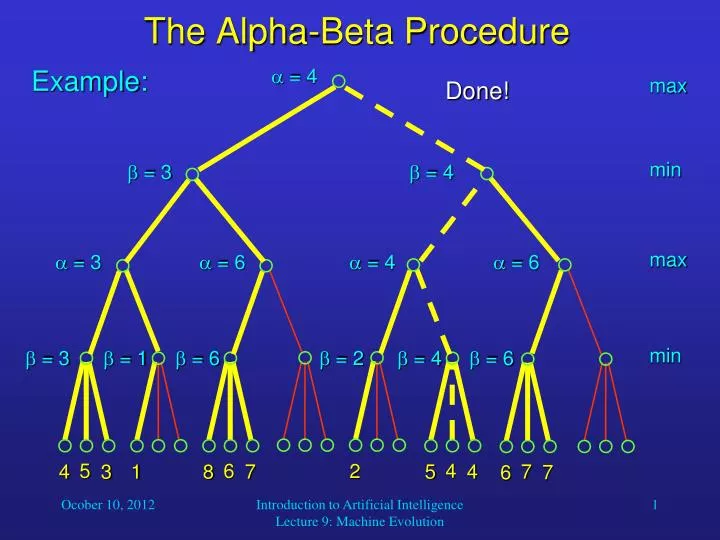
1. The Alpha-Beta Procedure Example:  = 4 max Done! min  = 3  = 4 max  = 3  = 6  = 4  = 6 min  = 3  = 1  = 6  = 2  = 4  = 6 5 6 4 2 4 3 1 8 7 5 4 7 6 7 Introduction to Artificial Intelligence Lecture 9: Machine Evolution

2. The Alpha-Beta Procedure • Can we estimate the efficiency benefit of the alpha-beta method? • Suppose that there is a game that always allows a player to choose among b different moves, and we want to look d moves ahead. • Then our search tree has bd leaves. • Therefore, if we do not use alpha-beta pruning, we would have to apply the static evaluation function Nd = bd times. Introduction to Artificial Intelligence Lecture 9: Machine Evolution

3. The Alpha-Beta Procedure • Of course, the efficiency gain by the alpha-beta method always depends on the rules and the current configuration of the game. • However, if we assume that somehow new children of a node are explored in a particular order - those nodes p are explored first that will yield maximum values e(p) at depth d for MAX and minimum values for MIN - the number of nodes to be evaluated is: Introduction to Artificial Intelligence Lecture 9: Machine Evolution

4. The Alpha-Beta Procedure • Therefore, the actual number Nd can range from about 2bd/2 (best case) to bd (worst case). • This means that in the best case the alpha-beta technique enables us to look ahead almost twice as far as without it in the same amount of time. • In order to get close to the best case, we can compute e(p) immediately for every new node that we expand and use this value as an estimate for the Minimax value that the node will receive after expanding its successors until depth d. • We can then use these estimates to expand the most likely candidates first (greatest e(p) for MAX, smallest for MIN). Introduction to Artificial Intelligence Lecture 9: Machine Evolution

5. The Alpha-Beta Procedure • Of course, this pre-sorting of nodes requires us to compute the static evaluation function e(p) not only for the leaves of our search tree, but also for all of its inner nodes that we create. • However, in most cases, pre-sorting will substantially increase the algorithm’s efficiency. • The better our function e(p) captures the actual standing of the game in configuration p, the greater will be the efficiency gain achieved by the pre-sorting method. Introduction to Artificial Intelligence Lecture 9: Machine Evolution

6. The Alpha-Beta Procedure • Even if you do not want to apply e(p) to inner nodes, you should at least do a simple check whether in configuration p one of the players has already won or no more moves are possible. • If one of the players has won, this simplified version of e(p) returns the value  or - if in configuration p the player MAX or MIN, respectively, has won. • It returns 0 (draw) if no more moves are possible. • This way, no unnecessary - and likely misleading - analysis of impossible future configurations can occur. Introduction to Artificial Intelligence Lecture 9: Machine Evolution

7. Timing Issues • It is very difficult to predict for a given game situation how many operations a depth d look-ahead will require. • Since we want the computer to respond within a certain amount of time, it is a good idea to apply the idea of iterative deepening. • First, the computer finds the best move according to a one-move look-ahead search. • Then, the computer determines the best move for a two-move look-ahead, and remembers it as the new best move. • This is continued until the time runs out. Then the currently remembered best move is executed. Introduction to Artificial Intelligence Lecture 9: Machine Evolution

8. How to Find Static Evaluation Functions • Often, a static evaluation function e(p) first computes an appropriate feature vector f(p) that contains information about features of the current game configuration that are important for its evaluation. • There is also a weight vector w(p) that indicates the weight (= importance) of each feature for the assessment of the current situation. • Then e(p) is simply computed as the dot product of f(p) and w(p). • Both the identification of the most relevant features and the correct estimation of their relative importance are crucial for the strength of a game-playing program. Introduction to Artificial Intelligence Lecture 9: Machine Evolution

9. How to Find Static Evaluation Functions • Once we have found suitable features, the weights can be adapted algorithmically. • This can be achieved, for example, with an artificial neural network. • So the biggest problem consists in extracting the most informative features from a game configuration. • Let us look at an example: Chinese Checkers. Introduction to Artificial Intelligence Lecture 9: Machine Evolution

10. Chinese Checkers • Move all your pieces into your opponent’s home area. • In each move, a piece can either move to a neighboring position or jump over any number of pieces. Introduction to Artificial Intelligence Lecture 9: Machine Evolution

11. Chinese Checkers • Sample moves for RED (bottom) player: Introduction to Artificial Intelligence Lecture 9: Machine Evolution

12. Chinese Checkers 8 7 7 4 5 6 6 6 5 4 • Idea for important feature: • assign positional values • sum values for all pieces of each player • feature “progress” is difference of sum between players 5 4 5 5 4 5 4 4 4 4 4 3 3 3 3 3 3 2 2 2 2 2 2 2 1 1 0 Introduction to Artificial Intelligence Lecture 9: Machine Evolution

13. Chinese Checkers • Another important feature: • For successful play, no piece should be “left behind” • Therefore add another feature “coherence”: Difference between the players in terms of the smallest positional value for any of their pieces. • Weights used in sample program: • 1 for progress • 2 for coherence Introduction to Artificial Intelligence Lecture 9: Machine Evolution

14. Isola • Your biggest programming assignment in this course will be the development of a program playing the game Isola. • In order to win the tournament and receive an incredibly valuable prize, you will have to write a static evaluation function that • assesses a game configuration accurately and • can be computed efficiently. Introduction to Artificial Intelligence Lecture 9: Machine Evolution

15. Isola • Rules of Isola: • Each of the two players has one piece. • The board has 77 positions which initially contain squares, except for the initial positions of the pieces. • A move consists of two subsequent actions: • moving one’s piece to a neighboring (horizontally, vertically, or diagonally) field that contains a square but not the opponent’s piece, • removing any square with no piece on it. • If a player cannot move any more, he/she loses the game. Introduction to Artificial Intelligence Lecture 9: Machine Evolution

16. Isola • Initial Configuration: Introduction to Artificial Intelligence Lecture 9: Machine Evolution

17. Isola • If in this situation O is to move, then X is the winner: If X is to move, he/she can just move left and remove the square between X and O, and also wins the game. Introduction to Artificial Intelligence Lecture 9: Machine Evolution

18. Isola • You can start thinking about an appropriate evaluation function for this game. • You may even consider revising the Minimax and alpha-beta search algorithm to reduce the enormous branching factor in the search tree for Isola. • We will further discuss the game and the Java interface for the tournament next week. Introduction to Artificial Intelligence Lecture 9: Machine Evolution

19. Let’s look at… • Machine Evolution Introduction to Artificial Intelligence Lecture 9: Machine Evolution

20. Machine Evolution • As you will see later in this course, neural networks can “learn”, that is, adapt to given constraints. • For example, NNs can approximate a given function. • In biology, such learning corresponds to the learning by an individual organism. • However, in nature there is a different type of adaptation, which is achieved by evolution. • Can we use evolutionary mechanisms to create learning programs? Introduction to Artificial Intelligence Lecture 9: Machine Evolution

21. Machine Evolution • Fortunately, on our computer we can simulate evolutionary processes faster than in real-time. • We simulate the two main aspects of evolution: • Generation of descendants that are similar but slightly different from their parents, • Selective survival of the “fittest” descendants, i.e., those that perform best at a given task. • Iterating this procedure will lead to individuals that are better and better at the given task. Introduction to Artificial Intelligence Lecture 9: Machine Evolution

22. Machine Evolution • Let us say that we wrote a computer vision algorithm that has two free parameters x and y. • We want the program to “learn” the optimal values for these parameters, that is, those values that allow the program to recognize objects with maximum probability p. • To visualize this, we can imagine a 3D “landscape” defined by p as a function of x and y. • Our goal is to find the highest peak in this landscape, which is the maximum of p. Introduction to Artificial Intelligence Lecture 9: Machine Evolution

23. Machine Evolution • We can solve this problem with an evolutionary approach. • Any variant of the program is completely defined by its values of x and y and can thus be found somewhere in the landscape. • We start with a random population of programs. • Now those individuals at higher elevations, who perform better, get a higher chance of reproduction than those in the valleys. Introduction to Artificial Intelligence Lecture 9: Machine Evolution

24. Machine Evolution • Reproduction can proceed in two different ways: • Production of descendants near the most successful individuals (“single parents”) • Production of new individuals by pairs of successful parents. Here, the descendants are placed somewhere between the parents. Introduction to Artificial Intelligence Lecture 9: Machine Evolution

25. Machine Evolution • The fitness (or performance) of a program is then a function of its parameters x and y: Introduction to Artificial Intelligence Lecture 9: Machine Evolution

26. Machine Evolution • The initial random population of programs could look like this: Introduction to Artificial Intelligence Lecture 9: Machine Evolution

27. Machine Evolution • Only the most successful programs survive… Introduction to Artificial Intelligence Lecture 9: Machine Evolution

28. Machine Evolution • … and generate children that are similar to themselves, i.e., close to them in parameter space: Introduction to Artificial Intelligence Lecture 9: Machine Evolution

29. Machine Evolution • Again, only the best ones survive and generate offspring: Introduction to Artificial Intelligence Lecture 9: Machine Evolution

30. Machine Evolution … until the population approaches maximum fitness. • … and so on… Introduction to Artificial Intelligence Lecture 9: Machine Evolution