Download
1 / 26
260 likes | 408 Views
Mode Selection. Determine when what component is running at what mode Mode selection is non-trivial Scheduler will be overwhelmed to determine component modes at the same time! Exploration space of all mode combinations is tremendous

E N D
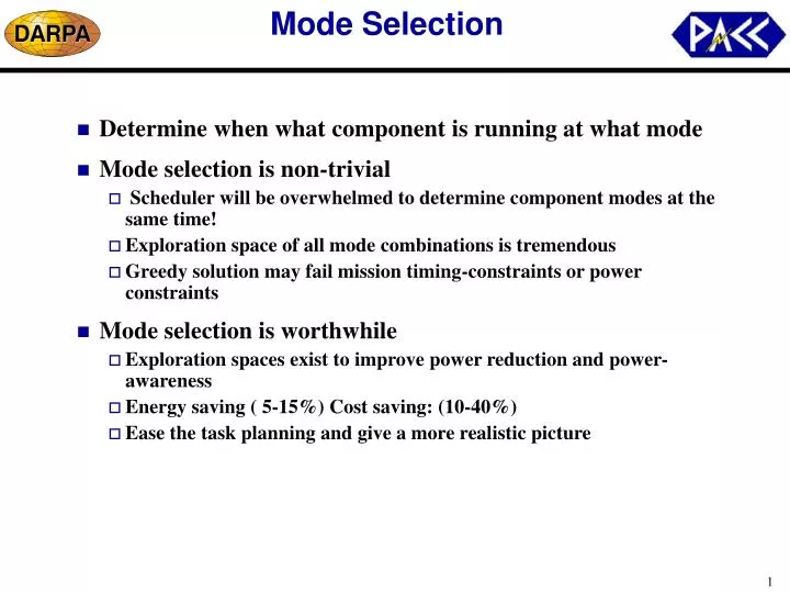
Mode Selection • Determine when what component is running at what mode • Mode selection is non-trivial • Scheduler will be overwhelmed to determine component modes at the same time! • Exploration space of all mode combinations is tremendous • Greedy solution may fail mission timing-constraints or power constraints • Mode selection is worthwhile • Exploration spaces exist to improve power reduction and power-awareness • Energy saving ( 5-15%) Cost saving: (10-40%) • Ease the task planning and give a more realistic picture
modified schedule Scheduler Mode Selector Initial schedule Power/timing number power profile Power/timing budget Power profile Power Estimator Power/timing budget Methodology and Design Flow • The whole picture - the integration of: • Power-aware scheduler • Mode selector • Power estimation/profiling tools • Static view
Application - Mars Rover • Mission-critical embedded system • Hard real-time system • Composed of COTS component • Electronic: µprocessor, µcontroller, memory,camera, scientific devices, ... • Mechanics/thermal: driving motor, steering motor, heaters, … • Power sources: solar panel, battery • Power/energy and performance constraints • Stringent max power constraint • Flexible min power constraint • Limited non-rechargeable energy sources • Global timing requirement • Limited working window during sol daytime • Timing constraint among tasks • Harsh and uncertain working environment • Extremely low temperature - affects component behaviors • Uncertain environment: winds/obstacles/rugged terrain
System Modeling High-level tasks • Component power model • Power modes with overheads • System timing model • Constraint graph • Inter-component model • Dependency graph • System parameters • Environment temperature • Surrounding terrain Component power model System timing model Inter-component model System constraints System parameters Schedule w/mode selection
Component Power Model • Component Power Modes • Power modes • Each mode has its own power and timing attributes • Constant • Profile • Function of system parameters • Complex component may have hierarchical modes • Microprocessor active-> cache on (off) ->cache settings • Microprocessor active-> voltage scaling • Microprocessor doze-> clock scaling • Microprocessor sleep • Overheads between mode changes • Power/energy overhead, e.g. preheating a motor, voltage scaling • Timing overhead between mode changes • Parameter-dependent overheads • Power/timing overheads are functions of system parameters, e.g. temperature, terrain • Both power and timing overhead can be parameter-dependent
Power: 2.2W Time: (-1.875*T+10)*(T<0) +10*(t>=0) off on Power: - 0.1225*T + 1.0 0W Power: 0.5W Time: 3 Component Model Examples • Examples of component model • Driving motor • Microprocessor (PowerPC 603e) Full power 4.0W 3.2W DPM 10 cycles - 10 cycles - 100us + 255 bus clocks + 10 cycles 10 cycles - 100us + 255 bus clocks + 10 cycles 10 cycles - Doze Sleep Nap 40mW 1.0W 70mW 3 cycles t1 + 3 cycles t1 + 3 cycles
10 A.s B.e System Timing Model • Constraint graph • Characterize the timing relationship between tasks • Model a task with two events • Start event • End event • Representation • Nodes: events of tasks • Directed edges and weights : timing relations between events • Edges between two events: • From start to end • From start to start • From end to start • From end to end • Weights on edges • Positive: “no earlier than” • Negative : “ no later than” End event of B should be no earlier than 10 time units after the start event of A -10 A.s B.s Start event of A should be no later than 10 time units after the start event of B
System Timing Modeling Example Haz: hazard detector Str: steering motor Drv: driving motor Cam: camera Ppc: processor Sci: scientific device Rf : radio frequency modem • Micro Rover example • Multiple resources • Timing constraints between tasks rf.s -5 5 -5 sci.e sci.s rf.e 5 1 -30 -5 str.s str.e ppc1.e ppc1.s 5 1 1 -5 -5 -10 5 1 cam.e haz.e drv.s drv.e cam.s 5 10 -5 5 haz.s
Inter-component Model • Dependency graph • Characterize power modes dependencies among components • Why dependency graph? • A distinction between functional modes v.s. resource modes • Functional modes:e.g. camera: high resolution, low resolution • Resource modes: voltage/clock scaling modes • A model to bridge the gap between two kinds of modes • Help prune out infeasible mode combinations from design space • Representation - directed graph • Nodes • Mode level graph • modes of component • Conjunctive operators: AND, OR, XOR, MUE ( mutual exclusion)… • Component level graph • components • Edges: • dependencies
Inter-component Modeling Example I str.off • Rover Example • Components: hazard detector, driving motor, steering motor • Constraints: hazard detector and the motors should not be working at the same time • Mode combinations haz.on Drv.off str.on OR Haz.off drv.on str.on drv.on MUE MUE str.off drv.off Haz: hazard detector Str: steering motor Drv: driving motor
Inter-component Modeling Example II A:ARM M:memory R: radio S: sensor • Micro Sensor Example • Components: processor, memory, RF, sensor • Constraints: • Processor is active when both radio and sensor is active • Memory is active only when processor is active • Microsensor architecture S.off AND A.sleep R.off S.on A.sleep A.idle XOR R.rx_tx R.rx A.active M.on A.idle A.sleep M.off
Inter-component Modeling Example II (cont’d) • Micro Sensor Example • Mode combinations given by MIT group: 5 combinations • Mode combination generated from dependency graph • Add constraint: • When sensor is off, all other component should be off (proactive) • Automatically obtain same results as MIT group Not given by MIT group M.off A.sleep M.off S.off
on off off off sleep sleep off off Mode Combination Enumeration- Using Dependency Graph Radio • Component level dependency graph • Obtain a component list by topological sorting • Each component is dependent upon predecessors only. • Enumerating modes • Working with cyclic graph • Mode level graph can’t have cycles • Break a cycle in component level graph by removing an edge • Topological sorting • When a component is dependent on its successors, let the last successor remember the component ARM Memory Sensor Sensor Radio ARM Memory idle off on idle off active on
System Parameters and Constraints • Parameters in system model • Temperature, terrain • Used to characterize components and their overheads • System Constraints • Maximum Power constraint • Constant or power profile (function of time) • Minimum Power constraint • Constant or power profile ( function of time) • Total energy constraint ( under working) • Mission time (mission deadline) Power consumption of Driving motor at different temperatures
System Power Representation • Schedule • Gantt Chart • Time view • Power view • Mode selection • Gantt chart • Tasks marked with mode settings • Added non-operating tasks • Idle intervals • mode change overheads • Power profile view
Component library System constraints schedule Mode selector Mode selections Problem Statement • Problem input • A schedule • Component library • System constraints • Problem output • Mode selection for the components/tasks • Problem statement • Find feasible mode selection for the tasks/idle intervals for the components that meets system power and timing constraints
Methodology and Work Flow • Exploration techniques • Backtracking • Cutting exploration space with multi-dimensional constraints • Two steps in design exploration: • Find feasible mode selection for operating tasks • Timing constraints • Constraint graph • Resource slacks • Mission deadline • Dependency between tasks • Dependency graph • Find feasible mode selections for idle intervals • System power/energy constraints: min, max, or power profile • Mode change overhead, both time and power overheads • Speedup techniques • Sorting component modes with power numbers
Application Example • Mars Rover • Behaviors and tasks • Moving around on Mars surface • Hazard detection, driving and steering • Communicating with the Lander • Taking pictures (IMP) • Performing scientific experiments (APXS, ASI/MET) • Components in the entire system • Hazard detector (HAZ), • Driving motor (DRV) • Steer motor (STR) • Radio frequency modem (RF) • Camera (CAM) • Microprocessor (PPC), • Micro-controller (MC) A schedule of the electronic subsystem of micro rover
Results - I • Non-Mode Selection solutions • Only two modes:On and off • Relaxed constraints: • Modes are selected to satisfy timing constraints • Power constraints may be violated • Mode change overheads are considered • Compare mode selection with non-mode selection • Mode selection energy saving: • From 3.7% to 11.9% • Average 8.7% • power constraints • Mode selection satisfies all max power constraints (14W) • Non-mode selection fails all max power constraints
Result II • Compare mode selection with non-mode selection • Cost saving: • Cost defined as energy above minimum power constraints • From 6.9% to 49.3% • average 26.5%
Exploring Different Working Scenarios • Explore different working scenarios and compare results • Three tasks • Moving around (MOV) • Taking picture (CAM) • Scientific experiment (SCI) • Three scenarios • A: MOV, CAM, SCI • B: CAM, MOV, SCI • C: CAM, SCI, MOV • Temperature profile is given as:
Result III • Different working scenarios have different energy consumption • Scenario C consumes 12% more energy than scenario A (by mode selection) • Mode selection always does better than simply two power modes( on&off)
Tool Prototype • Language • Python, Tkinter • Graphical User Interface • Features • Time window and power window • View tasks, overheads, power profile • Interactive command line • Dynamically load schedule, component library, or even algorithm • Interactive schedule modification • Interactive constraints modification • Incorporate with the scheduler (to be completed) • On-line help (to be completed)