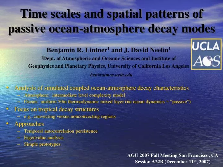
Time scales and spatial patterns of passive ocean-atmosphere decay modes

1. Time scales and spatial patterns of passive ocean-atmosphere decay modes Benjamin R. Lintner1 and J. David Neelin1 1Dept. of Atmospheric and Oceanic Sciences and Institute of Geophysics and Planetary Physics, University of California Los Angeles • Analysis of simulated coupled ocean-atmosphere decay characteristics • Atmosphere: intermediate level complexity model • Ocean: uniform 50m thermodynamic mixed layer (no ocean dynamics = “passive”) • Focus on tropical decay structures • e.g., convecting versus nonconvecting regions • Approaches • Temporal autocorrelation persistence • Eigenvalue analysis • Simple prototypes ben@atmos.ucla.edu AGU 2007 Fall Meeting San Francisco, CA Session A22B (December 11th, 2007)

2. Observed autocorrelation persistence Total Variability Days • e-folding time of gridpoint temporal autocorrelation (  p) estimated from the ERSST data set (1950-2000) • Mostly low values (< 100 days), except over the central/eastern Pacific, parts of the Atlantic and Indian Ocean basins • Long persistence associated with El Niño/Southern Oscillation ENSO Regressed

3. Quasi-equilibrim Tropical Circulation Model (QTCM) • Approximate analytic solutions for tropical convecting regions Convection constrains Tvertical structure of baroclinic P gradients vertical structure of v vertical structure of  • Implement analytic solutions for projection of primitive equations in a Galerkin-like expansion in the vertical • QTCM includes a full complement of GCM-like parameterizations (e.g., radiative transfer, surface turbulent exchange, Betts-Miller convection); is computationally efficient; and has been applied to multiple problems in tropical climate dynamics (e.g., ENSO teleconnections, monsoons, global warming,…) (Note: the version here has K =1.) See Neelin and Zeng, 2000; Zeng et al., 2000

4. QTCM Equations

5. Simulated p Days QTCM • Large spread in values (~50 days to > 300 days) • Relationship between mean precipitation (line contours) and persistence • Long persistence in SE tropical Pacific/Atlantic (weak convection) • Long persistence in ENSO source region • Implications for ENSO variability and/or characteristics? • Statistically significant spatial pattern correlation between models (r = 0.54) CCM3

6. Eigenvalue analysis • Interpretation of autocorrelation persistence ambiguous (e.g., single timescale only; local versus nonlocal influences?) • Eigenvalue analysis offers a simple way to estimate the modal nature of (slow) ocean-atmosphere decay • Approach:Partition the oceanic domain into N regions that form a N-dimensional subspace of SST anomalies. An SST perturbation (Ts) is applied to the jth region, and the anomalous surface heat flux in the ith region is computed (Fi). Thus, the time-evolution is: : Diagonal matrix of mixed layer depths (assumed equal) : Eigenvector matrix of cm-1G : Diagonal matrix with elements e-it, with i the eigenvalues of cm-1G

7. Eigenvalue example Days Eigenvalues/Decay Times Decay Time  i-1 • 35 basis regions (33 tropical; 2 extratropical) • Only ~3 modes have decay times substantially larger than the local decay times, estimated from the diagonal elements of G • Leading mode has most uniform spatial structure (as expected), but nonnegligible regional structure Local Decay Estimate  Gii-1 Mode # Mode 1 Loading

8. Decay time scaling • Approach:In 1D, assuming a homogeneous basic state and diagnostic frictional momentum balance (rxT = uuu), solve the thermodynamic equations and obtain a dispersion relationship of the form: Characteristic length scale: Days • For typical QTCM parameters, k0 1.5 • Relatively rapid timescales dominate tropical decay • Inclusion of cloud-radiative feedback (CRF) lowers local decay times by half, but has less impact on broader modes • CRF effect associated with shielding of the surface to incoming shortwave k0 = 0 (WTG limit: T uniform) k0 = 1 k0 = 2 k0 = 3 w/o CRF w/ CRF Mode #

9. Convecting-nonconvecting separation • Approach:Discretize equations subject to approximations (e.g., WTG limit) into N regions, with variable convection within a subset Nc and fully convecting in the rest, and perform eigenvalue analysis  1 (slow) Global, “G”; N-(Nc+1) (degenerate fast) Local Convecting, “LC”, and Nc (almost degenerate) Partially Convecting, “PC”, modes • (Inverse) decay time of LC/G modes insensitive/weakly sensitive to c, which indicates the frequency of convection in Nc • PC modes remain close to one another, esp. for large/small c • Relative insensitivity to areal extent of the nonconvecting region SST • Inverse decay time approaching G mode in nonconvecting limit (c = 0) Day-1 LC Nc ( = 2) boxes nonconvecting PC N ( = 8) boxes fully convecting G c

10. 2-box analogue • Approach:Replace N boxes by two: one fully convecting (of size fraction f1), the other partially convecting (of size fraction f2 = 1 - f1). The elements of G are: and the eigenvalues are given by: Notation: e.g., is T associated with 1K SST anom in box 1; 0K SST anom in box 2 • Facilitates straightforward analytic study of PC and G modes • A simplifying assumption in the 2-box case as shown is the strict QE limit (vanishing convective adjustment timescale), which accounts for the offset between N-box and 2-box solutions Day-1 f1 = 0.75 f1 = 0.75 f1 = 0.50 f1 = 0.33 PC PC G G c

11. Why nonconvecting regions decay slowly K Temperature c = 0 • In the fully convecting limit (c = 1), excitation of convective heating generates wave response • Strong horizontal spreading of the effect of the SST perturbation • Also, tight coupling of T and q • In the nonconvecting limit (c = 0), T and q largely decoupled, with little change in T • Weak spreading away from perturbation • Also in nonconvecting regions, evaporation balances moisture divergence (associated with large-scale descent) c = 0.25 c = 1 Box 2 Humidity f1

12. Eigenmode “blending” Day-1 • Increasing the horizontal damping/transport, such as through enhanced heat/moisture export of from the tropics through eddies, decreases G and PC mode decay times • Blending of eigenvector loadings occurs as the two eigenvalues approach one another in the limit of strong export • Plausible explanation for spatial nonuniformity seen in slowest decay mode(s) Eigenvalues unitless Eigenvectors Horizontal damping/transport (Wm-2K-1)

13. Thank you for listening! Acknowledgements: We thank J.C.H. Chiang for providing access to the CCM3 mixed layer simulation. This work was supported by NOAA grants NA04OAR4310013 and NA05)AR4311134 and NSF grant ATM-0082529. BRL further acknowledges partial financial support by J.C.H. Chiang and NOAA grant NA03OAR4310066. In press, Journal of Climate preprint available at: http://www.atmos.ucla.edu/~csi/