Download
1 / 27
300 likes | 540 Views
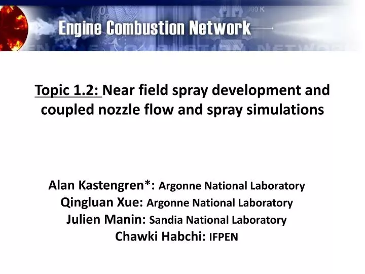
Topic 1.2: Near field spray development and coupled nozzle flow and spray simulations. Alan Kastengren*: Argonne National Laboratory Qingluan Xue: Argonne National Laboratory Julien Manin : Sandia National Laboratory Chawki Habchi : IFPEN. Modeling Part.

E N D
Topic 1.2: Near field spray development and coupled nozzle flow and spray simulations Alan Kastengren*: Argonne National Laboratory Qingluan Xue: Argonne National Laboratory Julien Manin: Sandia National Laboratory Chawki Habchi: IFPEN
Modeling Part • Facilitate dynamic coupling of in-nozzle flow and external spray approaches • Compare the different coupling approaches of in-nozzle flow and external spray • Study the capability of the different modeling approaches (Lagrangian-Eulerian, Eulerian-Eulerian) and CFD frameworks (RANS, LES, DNS) for the simulation of the primary atomization and the cavitation • Encourage high-fidelity simulations near nozzle sprays and liquid jet atomization
Spray A: Computational time (first 100µs) • Note: the computational domain size, initial conditions, and needle motions are different for the institutions
Computational domain (Spray A) Argonne CMT IFPEN Sandia UMASS • The inflow boundary conditions are specified at upstream for all simulations
Spray A (675) modeling results • Mass flow rate at the nozzle exit • Fuel spray penetration vs. time (0.1% liquid mass fraction) • Contour plots of projected density in the 0°plane at 0.1 and 0.5 ms after actual SOI • Projected fuel mass/density (ug/mm2) profiles across nozzle axis at 0.5 ms after SOI • x = 0.1, 0.6, 2, 6, and 10 mm downstream to nozzle exit • @ x= 0.6 and 6 mm, @ 0.75 ms and 1 ms after SOI • 2D contours of liquid volume fraction at x = 0.1, 0.6, 2, 6, 10 mm • Transverse integrated mass profiles at 0.5 ms after SOI: • x = 0.1 mm, 0.6 mm, 2 mm, 6 mm, and 10 mm • Mean droplet size (SMD) at x = 1, 4, 8 mm at 0.5 ms after SOI • Mean SMD at the above axial positions vs. axial position • Distributions of SMD vs. radial position at the above axial positions • Dynamics: peak projected density and Full Width Half Maximum (FWHM) of distribution at x = 0.1, 2, 6 mm from nozzle for entire duration of the injection event (in intervals of 20 μs)
Spray A: Predicted mass flow rate at nozzle exit Enlarged @ first 0.1ms • All simulations predict similar mass flow rates as the ROI from CMT’s Virtual generator • The transient process at the start of injection is different from the modeling groups since the minimum or fixed needle lift used are different • Starting from empty sac, initial LES penetration for IFPEN (up to 10 μs) compares well with the ROI from CMT’s generator, but it is oscillating; LES for UMass under-predicts The start of injection is defined as first evidence of liquid outside of the nozzle exit
Spray A: spray penetration • The data measured by Argonne and Sandia • Argonne, CMT and IFPEN: The liquid penetration defined by 0.1% mass fraction • Sandia: Mixture-fraction of 0.79 cut-off for the dense flow model • Initially Sandia simulations over-predict penetration but the liquid length is lower • CMT predict higher mass flow rate but lower penetration compared to Sandia • Argonne over-predict penetration due to high initial minimum needle lift Note: Sandia simulated conditions (Ambient=N2@900K and 60bar); Standard conditions for topic 1.2 are (Ambient=N2@303K and 20bar)
Spray A: projected mass density – 0.1ms ASOI Mass/area (μg/mm2) X-ray data Argonne RANS CMT IFPEN LES Sandia • All simulations predict quite different liquid jets • A dense liquid core near nozzle region is captured by all simulations • All simulations over-predict liquid penetration • RANS models tend to be overly diffusive compared to LES • LES over-predict the core length and some averaging to be comparable to x-ray results
Spray A: projected mass density – 0.5ms ASOI Mass/area (μg/mm2) X-ray Argonne Geometry RANS CMT UMASS LES IFPEN • At steady-state, the observations are consistent with earlier injection time (0.1ms) • LES simulation captures the fact that spray is off-axis, because IFPEN consider a more detailed geometry with finer mesh
Spray A: IFPEN calculation @ 0.5ms • Velocity vector plots in 3-D (left) and 2-D show the asymmetric distributions • Geometry effect on downstream spray predicted
Spray A: projected mass density – 0.5ms ASOI Argonne RANS Geometry CMT @0.25ms Sandia UMASS LES IFPEN • RANS simulations tend to over-predict radial diffusion; • LES simulations tend to over-predict liquid core length • IFPEN consider a more detailed geometry with finer mesh and predict off-axis spray
Spray A: 2-D (YZ) Liquid Volume Fraction (LVF) Argonne IFPEN Sandia X=0.6mm X=0.1mm X=2mm 0.5ms ASOI Geometry Others Tomographic Reconstruction from x-ray IFPEN RANS LES • Very high LVF (close to 1) are seen from Tomographic reconstruction x-ray data • RANS results are symmetric due to symmetric geometry used • Asymmetric liquid jet is shown from LES due to asymmetric geometry used • Low LVF (max=0.65) obtained LES results due to the presence of gaseous cavitation in the [0.1,2] mm region.
Spray A: Radial profiles of projected density density 0.5ms ASOI 0.5ms ASOI • 0 degree view from x-ray is asymmetric at all locations • Argonne and CMT use the same geometry, and fair comparison between the EE model is obtained • Sandia and UMass LES predict quite symmetric with the geometry used • All simulations capture the shape of the radial profile, however, significant differences in the peak values and tails (IFPEN GERM model predicts some gaseous cavitation in the [0.1,2] mm region) Note: The profiles from simulations are shifted to have the same phase as the x-ray data
Spray A: Radial profiles of projected density 0.5ms ASOI • Multiple realizations are necessary for LES to get smoother profiles • Significant difference between Argonne and CMT, although the similar EE model used (some difference in details) • Suggest to use the new geometry for the RANS cases in future work
Spray A: Projected fuel density 0.5, 0.75, 1.0 ms LES RANS • Argonne RANS predicts liquid jet reaches steady-state after 0.5 ms ASOI similar than x-ray experiments. • IFPEN Single-realization LES shows liquid jet reaches steady state after 0.5 ms, and may be at 0.75 ms
Spray A: Transverse Integrated Mass (TIM) 0.5ms ASOI • TIM increases with axial distance, all the simulations capture this trend • All simulations over-predicted the TIM which may be due to over dispersion in the radial direction • TIM at nozzle exit corresponds with the mass flow rate trends from topic 1.1 • CMT profile is not monotonic perhaps due to initial conditions
Spray A: peak density & FWHM vs. time Peak projected density FWHM • Similar peak values predicted by ANL and CMT at 0.1mm and 2.0mm, IFPEN under-predicted • We see variations from RANS results from CMT due to pressure wave and compressibility effect • Fluctuations are expected from LES@ SGS which may enhance primary atomization
Spray A: SMD at first 50 μs for IFPEN • Sub-microns droplets observed for IFPEN simulation which is consistent with x-ray measurement
Spray A: EE vs. LE at Argonne X-ray data Eulerian Lagrangian Projected mass density along spray axis • Eulerian model is better than traditional Lagrangian approach in the near nozzle region • Lagrangian simulations: 62.5μm minimum resolution, blob injection model, 300,000 parcels Mass-averaged velocity along axis
Spray B: Internal flow to external spray Phoenix geometry UMass contribution Hole 2 Hole 3 Hole 1 Mass fraction of gas • Hole # 3 has wider distribution
Spray B: spray velocity at 100 μs ASOI Hole #1 Hole #3 Argonne contribution Hole #2 CONVERGE reduced High-resolution geometry • Preliminary results for 3-D transient simulation at 10 microns resolution • Zoomed-in view shows holes #3 has wider spray compared to other holes • The effect of geometry, needle wobble, grid alignment and resolution to be investigated in the future work
Conclusions • Eulerian model is suitable for the coupling nozzle and near-field dense spray • For the first time, quantitative data on spray morphology in the near nozzle region was extracted from simulation • Significant insight from different simulation approaches were obtained when compared against experimental data • The Eulerian simulations seem to work better than Lagrangian simulations in the near nozzle region • A few key challenging areas for modeling: • Liquid compressibility • Temperature variation • Gas in the sac • Grid resolution • 2-D results are good and computationally cheap, needle off-axis motion and geometric asymmetries need 3-D simulations
Acknowledgements • All Contributors: • Argonne National Laboratory: Qingluan Xue, Michele Battistoni, SibenduSom • CMT - MotoresTérmicos: Pedro Martí, RaúlPayri • IFPEN: ChawkiHabchi, Rajesh Kumar • Sandia National Laboratories: GuilhemLacaze, Joseph C. Oefelein • University of Massachusetts Amherst: Maryam Moulai, David P. Schmidt