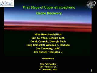
First Stage of Recovery in the Stratospheric Ozone Layer

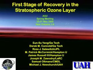
1. First Stage of Recovery in the Stratospheric Ozone Layer Eun-Su Yang/Georgia Tech Derek Cunnold/Georgia Tech Ross Salawitch/JPL Pat McCormick/Hampton U Jim Russell/Hampton U Joe Zawodny/LaRC Rich Stolarski/GSFC Rich McPeters/GSFC Sam Oltmans/CMDL Mike Newchurch/UAH Presented at AURA Science Team Meeting/Pasadena 2 March 2005

2. The ozone trend model [O3]t =  + t + [Seasonal terms] + [QBO periodic terms] + γ [F10.7]t + Nt  is the mean level,  is a linear trend coefficient, the seasonal terms represent the 12-, 6-, 4-, and/or 3-months cosine terms each with a time lag The QBO periodic terms consist of cosines with time lags to represent QBO signal with periods between 3 and 30 months excluding 12-, 6-, 4-,and/or 3-months terms. The traditional approach of using Singapore winds with a fitted lag produces similar results, but with less precise trend estimates and more fluctuations in the residuals. [F10.7]t is the F10.7-cm radio flux density which is used to provide a solar variation proxy. γ is a solar signal regression coefficient. Nt is the autocorrelated error term, for which a first order autoregressive process is assumed (Nt = a1Nt-1 + t). The t residuals, after removing the autoregressive component, a1Nt-1, are the residuals that are used to compute the cumulative sums of residuals described in Appendix B.

3. Ozone trend+residual and Cumulative Sums 60S-60N SAGE and MOD 30S-60N ground sites Green line represents constant ozone after 1997 2-sigma CUSUM [%] Envelope after 1997

4. 3 year lag wrt surface Inflection in 1997 Effective Equivalent Stratospheric Chlorine Photochemical model & EESC Fractional halogen loss of O3 constrained by: HALOE CH4 : used to specify Cly, Bry & NOy HALOE & SAGE H2O SAGE Surface Area HALOE & SAGE O3 and overhead O3 column Pre-UARS trends in H2O & CH4 based on SPARC & WMO Model constrained in this manner provides accurate description of measured ClO, NO, NO2, OH, and HO2 EESC fit to fractional halogen loss : 5 latitude bands: 50S to 50N Ignores Pinatubo period, which is not considered for trend analysis EESC fit to fractional halogen loss is a refinement that allows attribution analysis to consider effects of changing: • H2O • surface area • dynamically induced changes in Cly, etc.

5. Ozone trend+residual and Cumulative Sums 30N-60N Three data sets: SAGE Dobson-Brewer Merged TOMS/SBUV Merged TOMS/SBUV shows different “recovery” signature than SAGE and Dobson-Brewer

6. MOD trend+residual and Cumulative Sums 3 latitude bands Merged TOMS/SBUV

7. SAGE/HALOE and Halogen loss trend+residual and Cumulative Sums 3 latitude bands 18-25 km SAGE before 1992 HALOE after 1993 CUSUM [DU] - measure of departure from assumed linear trend, 1979 to 1997 Change in slope of residual ozone in 1997 is matched well by both: EESC fractional halogen loss

8. SAGE, ozonesonde, EESC fit 30N-60N 3 Altitude regions: Z > 25 km 18 to 25 km Z < 18 km EESC fit describes O3 changes for: Z > 25 km & 18 to 25 km but not for: Z < 18 km

9. Attribution to Dym and Chem: 2 layers Ozonesonde data, 30N-60N Chemical proxy = EESC Dynamical proxies = Temperature, Tropopause Height, PV 18 - 25 km : changes described by EESC Z < 18 km: changes described mainly by dynamical proxies

10. Polar processing effect on mid latitudes SAGE ozone residuals Polar proxy = V psc (inverted on plot) R = regression coefficient between SAGE ozone and Vpsc between February-April Effects of polar processing significant only below 18 km at 50-60N.

11. Vertical partitioning of trends and recovery

12. Vertical partitioning of trends and recovery

13. Conclusions Thickness of Earth’s stratospheric ozone layer stopped declining after about 1997. Signature of the observed changes above 18 km altitude is consistent with the timing of peak stratospheric halogen abundances. Confirms the positive effect of the Montreal Protocol and its amendments. Observed, large changes in stratospheric ozone below 18 km driven principally by changes in atmospheric dynamics. Changes are due to natural variability or due to changes in atmospheric structure related to anthropogenic climate change? Recent record during unusually low levels of stratospheric aerosol loading. Should a major eruption occur, will almost certainly lead to short periods of lower ozone. Data continuity across AURA period is critical to accurately diagnose changes and attribution of changes in stratospheric ozone.

14. Dedicated to Greg Reinsel1948 - 2004 Soft spoken gentleman. Conservative, rigorous scientist. Consummate statistician. Brought his considerable statistical expertise to the ozone community for 3 decades, primarily in analysis of Dobson and Umkehr ozone trends. Originated the idea of applying CUSUM technique to ozone measurements for early detection of changes in secular trends: The critical idea for the success of the work presented today.

15. http://nsstc.uah.edu/atmchem/ Support from NASA Earth Science Enterprise

16. SAGE/HALOE 40km trends and CUSUMs SAGE observations Northern Midlatitude Upper Stratosphere HALOE observations 2-σ confidence envelope Tropics Upper Stratosphere Southern Midlatitude Upper Stratosphere Measurements above projected trend