Regression

1. Regression • For classification the output(s) is nominal • In regression the output is continuous • Function Approximation • Many models could be used – Simplest is linear regression • Fit data with the best hyper-plane which "goes through" the points y dependent variable (output) x – independent variable (input) CS 478 - Regression

2. Regression • For classification the output(s) is nominal • In regression the output is continuous • Function Approximation • Many models could be used – Simplest is linear regression • Fit data with the best hyper-plane which "goes through" the points y dependent variable (output) x – independent variable (input) CS 478 - Regression

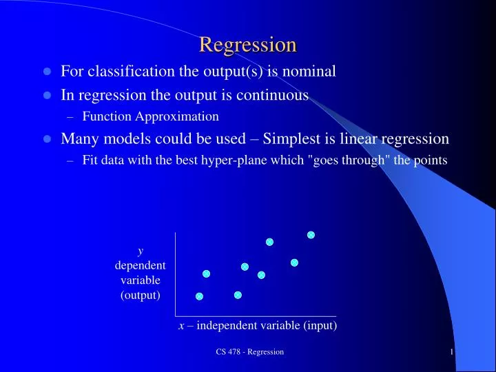
3. Regression • For classification the output(s) is nominal • In regression the output is continuous • Function Approximation • Many models could be used – Simplest is linear regression • Fit data with the best hyper-plane which "goes through" the points • For each point the differences between the predicted point and the actual observation is the residue y x CS 478 - Regression

4. Simple Linear Regression • For now, assume just one (input) independent variable x, and one (output) dependent variable y • Multiple linear regression assumes an input vector x • Multivariate linear regression assumes an output vector y • We will "fit" the points with a line • Which line should we use? • Choose an objective function • For simple linear regression we choose sum squared error (SSE) • S (predictedi – actuali)2 =S (residuei)2 • Thus, find the line which minimizes the sum of the squared residues CS 478 - Regression

5. How do we "learn" parameters For the 2-d problem (line) there are coefficients for the bias and the independent variable (y-intercept and slope) To find the values for the coefficients which minimize the objective function we take the partial derivates of the objective function (SSE) with respect to the coefficients. Set these to 0, and solve. CS 478 - Regression

6. Multiple Linear Regression • There is a closed form for multiple linear regression which requires matrix inversion, etc. • There are many different iterative techniques to solve it • One is the delta rule. We use an output node which is not thresholded (just does a linear sum) and iteratively apply the delta rule. • Delta rule will update towards the objective of minimizing the SSE, thus solving multiple linear regression. • There are many other linear regression approaches that give different results by trying to better handle outliers and other statistical anomalies CS 478 - Regression

7. Intelligibility • One nice advantage of linear regression models (and linear classification) is the potential to look at the coefficients to give insight into which input variables are most important in predicting the output • The variables with the largest magnitude have the highest correlation with the output • A large positive coefficient implies that the output will increase when this input is increased (positively correlated) • A large negative coefficient implies that the output will decrease when this input is increased (negatively correlated) • A small or 0 coefficient suggests that the input is uncorrelated with the output (at least at the 1st order) • Linear regression can be used to find best "indicators" • However, be careful not to confuse correlation with causality CS 478 - Regression

8. SSE and Linear Regression 3 3 • SSE chooses to square the difference of the predicted vs actual. Why square? • Don't want residues to cancel each other • Could use absolute or other distances to solve problem • S |predictedi – actuali|: • SSE leads to a parabolic error surface which is good for gradient descent • Would it choose the top or bottom line? • However, the squared error causes the model to be more highly influenced by outliers CS 478 - Regression

9. Anscombe's Quartet What lines "really" best fit each case? – different approaches CS 478 - Regression

10. Non-Linear Tasks • Linear Regression will not generalize well to the task below • Needs a non-linear surface • Could do a feature pre-process as with the quadric machine • For example, we could use an arbitrary polynomial in x • Thus it is still linear in the coefficients, and can be solved with delta rule, etc. • What order polynomial should we use? – Overfit issues occur as we'll discuss later CS 478 - Regression

11. Delta Rule for Classification x 1 z 0 x First consider the one dimensional case The decision surface for the perceptron would be any (first) point that divides instances Delta rule will try to fit a line through the target values which minimizes SSE and the decision point will be where the line crosses .5 for 0/1 targets Will converge to the one optimal line (and dividing point) in terms of this objective CS 478 - Regression

12. Delta Rule for Classification 1 z 0 x 1 z 0 x What would happen in this adjusted case for perceptron and delta rule and where would the decision point (i.e. .5 crossing) be? CS 478 - Regression

13. Delta Rule for Classification 1 z 0 x 1 z 0 x Leads to misclassifications even though the data is linearly separable For Delta rule the objective function is to minimize the regression line SSE, not maximize classification CS 478 - Regression

14. Delta Rule for Classification 1 z 0 x 1 z 0 x 1 z 0 x What would happen if we were doing a regression fit with a sigmoid/logistic curve rather than a line? CS 478 - Regression

15. Delta Rule for Classification 1 z 0 x 1 z 0 x 1 z 0 x Sigmoid fits many decision cases quite well! This is basically what logistic regression (LR) does. CS 478 - Regression

16. 1 0 Observation: Consider the 2 input perceptron case. Note that the output z is a function of 2 input variables for the 2 input case (x1, x2), and thus we really have a 3-d decision surface, yet the decision boundary is still a line in the 2-d input space. Delta rule would fit a regression plane to these points with the decision line being that line where the plane went through .5. What would logistic regression do?

17. CS 478 - Regression

18. Logistic Regression • One commonly used algorithm is Logistic Regression • Assumes that the dependent variable is binary • Often the case in medical studies and other studies. (Have disease or not, survive or not, accepted or not, etc.) • Logistic regression fits the data with a sigmoidal/logistic curve and outputs an approximation of the probability of the output given the input CS 478 - Regression

19. Logistic Regression Example • Age (X axis, independent variable) – Data is fictional • Heart Failure (Y axis, 1 or 0, dependent variable) • Could use value of regression line as a probability approximation • Extrapolates outside 0-1 and not as good empirically • Sigmoidal curve to the right gives empirically good probability approximation and is bounded between 0 and 1 CS 478 - Regression

20. Logistic Regression Approach Learning • Transform initial input probabilities into log odds (logit) • Do a standard linear regression on the logit values • This effectively fits a logistic curve to the data, while still just doing a linear regression with the transformed input (ala quadric machine, etc.) Generalization • Find the value for the new input on the logit line • Transform that logit value back into a probability CS 478 - Regression

21. Non-Linear Pre-Process to Logit (Log Odds) Cured 1 prob. Cured Not Cured 0 0 10 20 30 40 50 60 0 10 20 30 40 50 60 CS 478 - Regression

22. Logistic Regression Approach 1 1 prob. Cured prob. Cured 0 0 0 10 20 30 40 50 60 0 10 20 30 40 50 60 • Could use linear regression with the probability points, but that would not extrapolate well • Logistic version is better but how do we get it? • Similar to Quadric we do a non-linear pre-process of the input and then do linear regression on the transformed values – do a linear regression on the log odds - Logit CS 478 - Regression

23. Non-Linear Pre-Process to Logit (Log Odds) Cured 1 prob. Cured Not Cured 0 0 10 20 30 40 50 60 0 10 20 30 40 50 60 CS 478 - Regression

24. Regression of Log Odds +2 0 -2 0 10 20 30 40 50 60 1 prob. Cured 0 • y = .11x – 3.8 - Logit regression equation • Now we have a regression line for log odds (logit) • To generalize, we interpolate the log odds value for the new data point • Then we transform that log odds point to a probability: p = elogit(x)/(1+elogit(x)) • For example assume we want p for dosage = 10 • Logit(10) = .11(10) – 3.8 = -2.7 • p(10) = e-2.7/(1+e-2.7) = .06 [note that we just work backwards from logit to p] • These p values make up the sigmoidal regression curve (which we never have to actually plot) CS 478 - Regression

25. Summary Linear Regression and Logistic Regression are nice tools for many simple situations Intelligible results When problem includes more arbitrary non-linearity then we need more powerful models which we will introduce These models are commonly used in data mining applications and also as a "first attempt" at understanding data trends, indicators, etc. CS 478 - Regression