Download
1 / 24
240 likes | 370 Views
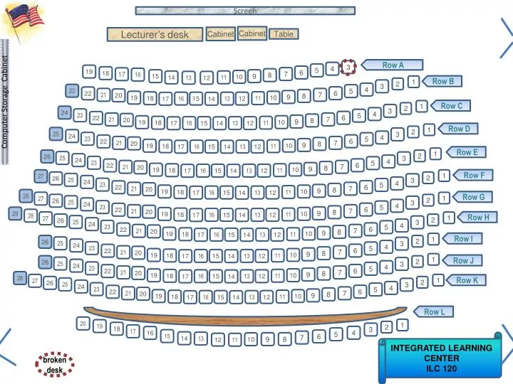
Screen. Cabinet. Cabinet. Lecturer’s desk. Table. Computer Storage Cabinet. Row A. 3. 4. 5. 19. 6. 18. 7. 17. 16. 8. 15. 9. 10. 11. 14. 13. 12. Row B. 1. 2. 3. 4. 23. 5. 6. 22. 21. 7. 20. 8. 9. 10. 19. 11. 18. 16. 15. 13. 12. 17. 14. Row C. 1. 2.

E N D
Screen Cabinet Cabinet Lecturer’s desk Table Computer Storage Cabinet Row A 3 4 5 19 6 18 7 17 16 8 15 9 10 11 14 13 12 Row B 1 2 3 4 23 5 6 22 21 7 20 8 9 10 19 11 18 16 15 13 12 17 14 Row C 1 2 3 24 4 23 5 6 22 21 7 20 8 9 10 19 11 18 16 15 13 12 17 14 Row D 1 2 25 3 24 4 23 5 6 22 21 7 20 8 9 10 19 11 18 16 15 13 12 17 14 Row E 1 26 2 25 3 24 4 23 5 6 22 21 7 20 8 9 10 19 11 18 16 15 13 12 17 14 Row F 27 1 26 2 25 3 24 4 23 5 6 22 21 7 20 8 9 10 19 11 18 16 15 13 12 17 14 28 Row G 27 1 26 2 25 3 24 4 23 5 6 22 21 7 20 8 9 29 10 19 11 18 16 15 13 12 17 14 28 Row H 27 1 26 2 25 3 24 4 23 5 6 22 21 7 20 8 9 10 19 11 18 16 15 13 12 17 14 Row I 1 26 2 25 3 24 4 23 5 6 22 21 7 20 8 9 10 19 11 18 16 15 13 12 17 14 1 Row J 26 2 25 3 24 4 23 5 6 22 21 7 20 8 9 10 19 11 18 16 15 13 12 17 14 28 27 1 Row K 26 2 25 3 24 4 23 5 6 22 21 7 20 8 9 10 19 11 18 16 15 13 12 17 14 Row L 20 1 19 2 18 3 17 4 16 5 15 6 7 14 13 INTEGRATED LEARNING CENTER ILC 120 9 8 10 12 11 broken desk
MGMT 276: Statistical Inference in ManagementRoom 120 Integrated Learning Center (ILC)Fall, 2012 Welcome
Use this as your study guide By the end of lecture today9/11/12 Value of Peer Review Correlational methodology Strength of correlation versus direction Positive versus Negative correlation Strong, versus Moderate versus Weak correlation Correlation does not imply causation(No “quasi-experimental” design can provide evidence of cause-and-effect relationship)
Homework due - (September 13th) On class website: please print and complete homework assignment # 4 Please double check – Allcell phones other electronic devices are turned off and stowed away
Review of Homework Worksheet On Tuesday Homework Reports must be complete, stapled, and polished
Peer review Please exchange questionnaires with someone (who has same TA as you) and complete the peer review handed out in class You have 10 minutes Peer review is an important skill in nearly all areas of business and science. Please strive to provide productive, useful and kind feedback as you complete your peer review
Review of Homework Worksheet Hand in the peer review with the questionnaire *Hand them in together*
Schedule of readings Before next exam: Please read chapters 1 - 4 & Appendix D & E in Lind Please read Chapters 1, 5, 6 and 13 in Plous Chapter 1: Selective Perception Chapter 5: Plasticity Chapter 6: Effects of Question Wording and Framing Chapter 13: Anchoring and Adjustment
Designed our study / observation / questionnaire Collected our data Organize and present our results
Scatterplot displays relationships between two continuous variables Correlation: Measure of how two variables co-occur and also can be used for prediction Range between -1 and +1 The closer to zero the weaker the relationship and the worse the prediction Positive or negative
Correlation Range between -1 and +1 +1.00 perfect relationship = perfect predictor +0.80 strong relationship = good predictor +0.20 weak relationship = poor predictor 0 no relationship = very poor predictor -0.20 weak relationship = poor predictor -0.80 strong relationship = good predictor -1.00 perfect relationship = perfect predictor
Positive correlation: as values on one variable go up, so do values for the other variable Negative correlation: as values on one variable go up, the values for the other variable go down Height of Mothers by Height of Daughters Height ofMothers Positive Correlation Height of Daughters
Positive correlation: as values on one variable go up, so do values for the other variable Negative correlation: as values on one variable go up, the values for the other variable go down Brushing teeth by number cavities BrushingTeeth Negative Correlation NumberCavities
Perfect correlation = +1.00 or -1.00 One variable perfectly predicts the other Height in inches and height in feet Speed (mph) and time to finish race Positive correlation Negative correlation
Correlation The more closely the dots approximate a straight line,(the less spread out they are) the stronger the relationship is. Perfect correlation = +1.00 or -1.00 One variable perfectly predicts the other No variability in the scatterplot The dots approximate a straight line
Correlation does not imply causation Is it possible that they are causally related? Yes, but the correlational analysis does not answer that question What if it’s a perfect correlation – isn’t that causal? No, it feels more compelling, but is neutral about causality Number of Birthdays Number of Birthday Cakes
Positive correlation: as values on one variable go up, so do values for other variable Negative correlation: as values on one variable go up, the values for other variable go down Number of bathrooms in a city and number of crimes committed Positive correlation Positive correlation
Linear vs curvilinear relationship Linear relationship is a relationship that can be described best with a straight line Curvilinear relationship is a relationship that can be described best with a curved line
Correlation - How do numerical values change? http://neyman.stat.uiuc.edu/~stat100/cuwu/Games.html http://argyll.epsb.ca/jreed/math9/strand4/scatterPlot.htm Let’s estimate the correlation coefficient for each of the following r = +.80 r = +1.0 r = -1.0 r = -.50 r = 0.0
This shows the strong positive (.8) relationship between the heights of daughters (measured in inches) with heights of their mothers (measured in inches). 48 52 5660 64 68 72 Both axes and values are labeled Both axes and values are labeled Both variables are listed, as are direction and strength Height of Mothers (in) 48 52 56 60 64 68 72 76 Height of Daughters (inches)
Break into groups of 2 or 3 Each person hand in own worksheet. Be sure to list your name and names of all others in your group Use examples that are different from those is lecture 1. Describe one positive correlation Draw a scatterplot (label axes) 2. Describe one negative correlation Draw a scatterplot (label axes) 3. Describe one zero correlation Draw a scatterplot (label axes) 4. Describe one perfect correlation (positive or negative) Draw a scatterplot (label axes) 5. Describe curvilinear relationship Draw a scatterplot (label axes)
Both variables are listed, as are direction and strength Both axes and values are labeled Both axes and values are labeled This shows the strong positive (.8) relationship between the heights of daughters (measured in inches) with heights of their mothers (measured in inches). 48 52 5660 64 68 72 1. Describe one positive correlation Draw a scatterplot (label axes) Height of Mothers (in) 2. Describe one negative correlation Draw a scatterplot (label axes) 48 52 56 60 64 68 72 76 Height of Daughters (inches) 3. Describe one zero correlation Draw a scatterplot (label axes) 4. Describe one perfect correlation (positive or negative) Draw a scatterplot (label axes) 5. Describe curvilinear relationship Draw a scatterplot (label axes)
Thank you! See you next time!!