Download
1 / 47
520 likes | 1.07k Views
Surface Water Hydrology. Summarized in one equation. V = velocity, fps or m/s A = channel cross-sectional area, sf or m 2. A. V. Stream Discharge (Q). Fundamental stream variable Cubic feet/second (cfs, ft -3 sec -1 ) Q=V*A Velocity (ft/sec) * Channel area (ft 2 ) Instantaneous.

E N D
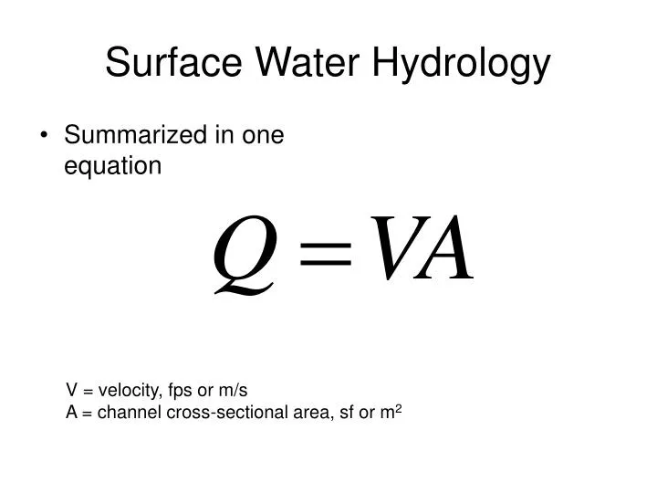
Surface Water Hydrology • Summarized in one equation V = velocity, fps or m/s A = channel cross-sectional area, sf or m2
A V Stream Discharge (Q) • Fundamental stream variable • Cubic feet/second(cfs, ft-3sec-1) • Q=V*A • Velocity (ft/sec) * • Channel area (ft2) • Instantaneous
Streamflow Measurement Figure 11.30
USGS Midsection MethodQ = ΣQi whereQi = (ui * di) * {( bi+1 – bi-1)/2} For d 4 use (b5-b3)/2
http://www.caf.wvu.edu/~forage/streamflow/estimat.htm Measure velocity at .6 x depth, as measured from the water surface For deep channels, measure velocity at 0.2 x depth and 0.8 x depth, from WS
Case Study: Yellowstone River at Livingston, MT • Manually measured occasionally to define rating curve: Q=VA • Continuously monitored: stage http://water.usgs.gov/waterwatch/
Yellowstone River II • Synthesized for floods / droughts • Summarized for risk / geomorphic work
Probability distribution functions of flood flow events • Theoretical distributions • Gumbel • Log Pearson type III (used in “Guidelines for calculation of flood flow frequency”, Water Resources Council Bulletin 17B) • Weibull
the distribution of the maximum of a number of samples Gumbel distribution • Used to describe annual flow events • Fits an extreme value distribution to flood data by assuming the annual flood is the largest of a sample of 365 possible values per year • Exceedence probability = 1-F(x)
Log Pearson type III distribution • Exceedence probabilities are estimated using a normal distribution with adjustments for skewness of the flow series • Flow values are transformed to logarithmic values • Average and standard deviation of the transformed values, and estimates of the skewness of the distribution are used to estimate the flood flow of a given recurrence interval • K value = f(skew value, desired recurrence interval) • Skew value = f(number of years of record)
Log Pearson type III distribution • Step 1: Transform flow data to log domain • Step 2: Calculate mean and standard deviation of log-transformed data set • Step 3: Calculate weighted skew • G = station skew • G-bar = generalized skew (from Plate 1 of Bull. 17B) • MSE = mean square error of each skew (from pgs. 13-14 of Bull. 17B)
Log Pearson type III distribution • Step 4: Using weighted skew and return interval of interest (e.g. 2 yr flood), look up type III deviate, K, in Appendix 3, Bulletin 17B • Calculate log of flow of desired return interval • E.g. at Blacksmith Fork nr. Hyrum, UT • log(Q2)=mean(log(Q’s))+K*standard deviation(log(Q’s)) • log(Q2)=2.64+(0.06)*(0.31) • Q2 = 455 cfs
Weibull distribution • Also called “plotting position”, p • Estimated cumulative probabilities • implies the largest observed value is the max possible value of the distribution • Sort n data from smallest to largest, assign a rank m, to the sorted data, and use m and n to calculate an empirical cumulative probability • Recurrence interval • 1/p
Weibull Distribution Discharge Value Rank , m Recurrence interval 10,000 1 (n+1/m) 6,200 2 5,000 3 500 50 m n Q Return Interval
A comparison of Gumbel, log Pearson type III, and Weibull distributions: calculation of Q2
What if there isn’t a gaging station? • Predict discharge from physiographic variables • drainage area, annual precip. (inches), % forested area, • Q = f(A) • SW Montana: • Q2 = 2.48 A0.87 (HE+10)0.19 • Omang, 92; USGS WRIR 92-4048
Linear Regression • Method of determining correlation between 2 (or more) variables • The quantity r, called the linear correlation coefficient, measures the strength and the direction of a linear relationship between two variables • The coefficient of determination, r 2,is useful because it gives the proportion of the variance (fluctuation) of one variable that is predictable from the other variable • It is a measure that allows us to determine how certain one can be in making predictions from a certain model/graph • The coefficient of determination is the ratio of the explained variation to the total variation • For example, if r = 0.922, then r2 = 0.850, which means that 85% of the total variation in y can be explained by the linear relationship between x and y (as described by the regression equation). The other 15% of the total variation in y remains unexplained.
You have determined that more than 23.4” of annual rainfall will result in a net Economic loss for your crop. Now, you need to predict How often this will occur.
Weibull Probability of Occurrence, Fa (%)= n 100 * y+1 n = the rank of each event y = the total number of events For Example: Year 1938--23.4 in--Rank #3 100 (3) = 15.0 % 20
Hazen Probability of Occurrence, Fa (%)= 100 (2n-1) 2y n = the rank of each event y = the total number of events For Example: Year 1938--23.4 in--Rank #3 100 (2*3-1) = 12.5% 2*20
100 Return Period= Fa Fa= probability of occurrence (%) For Example: Year 1938-- Fa= 12.5 100 = 8 yrs OR 100/15 = 6.7 yrs 12.5
Peak Streamflow for the Nation USGS 06043500 Gallatin River near Gallatin Gateway MT Fa(%) = 100* (n/y+1) Recurrence Interval (Return Period) = 100/Fa Using the entire 82 yrs of record, R.I.(9160) = 82 yrs R.I.(5500) = 2.4 yrs 16 yrs 2.7 yrs What’s the recurrence interval of the largest flood of the last 15 yrs? What’s the recurrence interval of the 2009 runoff peak?
Other types of flood predictions: fish migration flows • Estimation of Migration Flows during High Flow Periods • The magnitude of migration flows during high flow periods was estimated for the Upper Main and South Fork Red River watersheds using the 10 percent exceedance flow determined for the April to June period for each year of available data. • The April to June period was based on migration timing of steelhead trout and westslope cutthroat trout. • Mean daily flow data for April, May, and June for each year of record was sorted from largest to smallest. A rank was then assigned to the sorted data to calculate an empirical cumulative probability. • The high flow for migration was estimated as the flow at which the probability that a given flow will be equaled or exceeded is 10 percent. • A second estimate of high flows for migration was determined as 50 percent of the 2-year flood flow. The 2-year flood, as determined using the Log Pearson Type III distribution, was used to estimate migration flows during high flow periods.
Estimation of Migration Flows during Low Flow Periods • The magnitude of migration flows during low flow periods was estimated for the Upper Main and South Fork Red River watersheds using the 95 percent exceedance flow determined using data for August and September. • The August through September timing was based on spawning timing of chinook salmon and bull trout in the Newsome Creek watershed. • Mean daily flow data for August and September for each year of record was sorted from largest to smallest. • A rank was then assigned to the sorted data to calculate an empirical cumulative probability. • The low flow for migration was estimated as the flow at which the probability that a given flow will be equaled or exceeded of 95 percent of the time. • A second estimate of low flows for migration was determined by using the 7-day average for mean daily flow in August and September. For each year of record, a 7-day average was calculated for flows in August and September. The minimum 7-day average for each year was selected as the 7-day average for that year.