Download
1 / 62
620 likes | 824 Views
COMP4048 Planar and Orthogonal Graph Drawing Algorithms. Richard Webber National ICT Australia. Lecture Overview. Planarity Testing Planarity Tessellation Drawings Visibility Drawings Polyline Drawings Orthogonal Drawings via Visibility Drawings Orthogonal Drawings via Network Flow

E N D
COMP4048Planar and Orthogonal Graph Drawing Algorithms Richard WebberNational ICT Australia
Lecture Overview • Planarity • Testing Planarity • Tessellation Drawings • Visibility Drawings • Polyline Drawings • Orthogonal Drawings via Visibility Drawings • Orthogonal Drawings via Network Flow • Degree > 4 • Bend Stretching • Degree > 4 again
Planarity • A graph is planar if it can be drawn such that no edges cross • A drawing is planar if it is drawn with no edges crossing
Planarity • Straight-line drawing with no edge crossings = Fáry Drawing (Fáry 1948) • 2D Fáry Drawing = Planar (Graph) Drawing • Planar Drawing Planar Embedding Planar Graph • Plane Graph (drawing) = 2d
Planarity • Simple Planar Embedding n + f = m + 2 m = O(n) and f = O(n) m 3n-6 Euler (http://www-history.mcs.st-andrews.ac.uk/Biographies/Euler.html)
Testing Planarity • (Di Battista et al. 1999, Goldstein 1963) • Trees and SP Digraphs = planar • Graph = planar connect components = planar • Connect components = planar biconnected components = planar • Biconnected two vertex-disjoint paths
Testing Planarity • Find a cycle C in G (biconnected cycle must exist) • Decompose remaining edges into piecesPi • Connected without passing vertices of C • Incident vertices in C are attachments of Pi • If C 2+ pieces then C is separating • If C 1 piece then C is non-separating • C non-separating and P1 a path separating C
Testing Planarity • Each piece must lie entirely inside or outsideC • Two pieces interlace if they cannot both be inside (outside) C without breaking planarity • Interlacement graphI of Gwith respect toC • Vertices = pieces of G • Edges between interlacing pieces
Testing Planarity • Biconnected G with cycle C is planar iff • For each piece P, P’ = P C is planar; and • Interlacement graph Iis bipartite • Planarity of P’ determined recursively
Testing Planarity • Compute piece of G with respect to C • For each non-path piece P • P’ = P C • C’ = cycle of P’by replacing C between consecutive attachments with a path through P • Recursively test P’ with C’ – return if “non-planar” • Compute interlacement graph I • Return “non-planar” if I not bipartite • Return “planar”
Testing Planarity • Computing pieces and finding C’: O(n) • Computing I and testing bipartite: O(n2) • Each invocation = O(n2), O(n) invocations O(n3) running time • Can be improved to O(n) (Hopcroft+Tarjan 1974) • Can construct planar embedding • use bipartite interlacement graph to alternate inside/outside pieces • path-pieces trivially inserted • non-path-pieces constructed recursively
Planar st-Graphs • (Di Battista et al. 1999, Lempel et al. 1967) • Digraphs only • s = source, t = sink – only one of each • Add dummies if needed • Topological numbering – number(v) for v V such that (u, v) E number(v) > number(u) • Topological sorting – numbering [0..n-1] • For weighted edges number(v) number(u) + weight(u, v) • number(s) = 0; number(v) by max over BFS • optimal in O(n + m) time
Planar st-Graphs • F = faces of planar st-graph G such that external face split: left s* and right t* • orig(e), dest(e), left(e), right(e) • left(v), right(v), orig( f ), dest( f ) • orig(v) = dest(v) = v; left( f ) = right( f ) = f • G* = ( F, { ( left(e), right(e) ) | e E } ) • G* is also planar st-graph
Tessellation Drawings • (Di Battista et al. 1999, Tamassia+Tollis 1989) • Vertices / Edges / Faces = Objects • Object o drawn as a rectangle (o) • Possibly degenerate • (o1) (o2) = • Union over allo V E F = rectangle • (o)s horizontally adjacent os left/right • (o)s vertically adjacent os orig/dest
Tessellation Drawings • G* from G • Topological numbering Y of G • Topological numbering X of G* • For each o V E F • xL(o) = X(left(o)) • xR(o) = X(right(o)) • yB(o) = Y(orig(o)) • yT(o) = Y(dest(o)) • O(n) time and O(n2) area
Visibility Drawings • (Di Battista et al. 1999, Tamassia+Tollis 1986) • Vertices = Horizontal lines • Edges = Vertical lines • Intersections only where edges meet end-points • Tessellation Drawing Visibility Drawing • degenerate vertices, non-degenerate faces
Visibility Drawings • G* from G • weight(e) = 1 – Optimal topological numbering Y of G • weight(e*) = 1 – Optimal topological numbering X of G* • For each v V • y(v) = Y(v); xL(v) = X(left(v)); xR(v) = X(right(v))-1 • For each e E • x(e) = X(left(e)); yB(e) = Y(orig(e)); yT(e) = Y(dest(e)) • O(n) time and O(n2) area
Constrained Visibility • (Di Battista et al. 1999, Di Battista et al. 1992) • Identify non-intersecting pathsiin G • No common edges • No “crossings” • Can “touch” at vertices
Constrained Visibility • Set of paths covers G–Add single-edge paths • Duplicate each path, adding faces to G* gives G • weight(e) = 1, Y(s) = 0 – Optimal topological numbering Y of G • weight(e*) = 0.5, X(s*) = -0.5 – Optimal topological numbering X of G
Constrained Visibility • For each : for eache • x(e) = X() • yB(e) = Y(orig(e)) • yT(e) = Y(dest(e)) • For each v V • y(v) = Y(v) • xL(v) = minv X() • xR(o) = maxv X() • O(n) time and O(n2) area
Polyline Drawings • (Di Battista et al. 1999, Di Battista et al. 1992) • Construct a visibility drawing • Place vertex vi at an arbitrarypi on its line segment • Draw short edge (vi, vj) as line pipj • Draw long edge (vi, vj) as polyline pi (x(u, v), yu+1) (x(u, v), yv-1) pj
Polyline Drawing • Place vertex at mid-point of its line segment • O(n) time and O(n2) area • 6n-12 bends (2 per edge)
Polyline Drawing • Place vertex above long edges if they exist • O(n) time and O(n2) area • (10n-31)/3 bends
Polyline Drawing • Use constrained visibility • Place vertex on path • O(n) time and O(n2) area • 4n-10 bends
Orthogonal via Visibility • (Di Battista et al. 1999) • Input = planar st-graph • Create subpaths v for v {s,t} • 2 incoming edges leftmost-inrightmost-out • 1 or 3 incoming edges median-inmedian-out
Orthogonal via Visibility • Unify subpaths with common edges to give • Apply Constrained-Visibilityalgorithm
Orthogonal via Visibility • Create orthogonal drawing • Place vertex v {s,t} on path v • Place s(t) on path of median of out (in) edges • Routes general edges via paths • Route s(t) edges as …
Orthogonal via Visibility • O(n) time, O(n2) area, 2n+4 bends
Orthogonal via Network Flow • (Di Battista et al. 1999, Tamassia 1987) • Visibility guarantees O(1) bends per edge • Want to minimise total bends for embedding • minimising over all embeddings in NP-hard • Represent angles as a commodity • Produced by vertices, consumed by faces, transferred by bends • Apply a cost to each bend • Minimising bends = minimising cost of flow!
Orthogonal via Network Flow • Replace each (undirected) edge (u, v) with two darts(u, v) and (v, u) • dart = counterclockwise for ff is on left • (u, v)·/2 = angle from dart (u, v) to next dart counterclockwise about u • (u, v) = number of “left” bends in (u, v) • Orthogonal representation = all (, ) • Same representation same number bends
Orthogonal via Network Flow • Network Nsuch that… • Source (sink) v produces (consumes) (v) • Arc (u, v) has • Lower bound (u, v) • Capacity (u, v) • Cost (u, v) • Flow (u, v) such that (u, v) (u, v) (u, v) • Sum into v {s,t} = sum out • Cost of flow in N = sum all (u, v)·(u, v)
Orthogonal via Network Flow • Embed Graph G into Network N by… • Nodes of N = vertices and faces of G • Vertex-node v produces (v) = 4 • Internal face-node f consumes (f) = 2a(f)-4 • External face-node f consumes (f) = 2a(f)+4 • a(f) = number vertex-angles in face f
Orthogonal via Network Flow • Dart (u, v) with left (right) face f (g) • arc (u, f): (u, f) = 1, (u, f) = 4, (u, f) = 0 (u, v) • arc (f, g): (f, g) = 0, (f, g) = , (f, g) = 1 (u, v)
Orthogonal via Network Flow • Construct N from G – O(n) time • Compute minimum cost flow for N – O(n2 log n) (Ahuja et al. 1993) or O(n7/4 log n) (Garg+Tamassia 1997) time • Map Nto orthogonal representation for G – O(n) time
Orthogonal via Network Flow • To map orthogonal representation to drawing… • Divide the faces into rectangles • e corner(e) next(e) – counterclockwise • turn(e) = +1 (left), 0 (straight), –1 (right) • front(e) = 1st next(e’) s.t. sum e..e’ = +1 • If turn(e) = –1 then insert • Vertex project(e) in front(e) • Edge extend(e) = (corner(e), project(e))
Orthogonal via Network Flow • External face by enclosing in a rectangle • Total O(n+b) time – b = number of bends
Orthogonal via Network Flow • Assign edge lengths • Minimising lengths/area – compaction • Interior rectangles: (u, v) 2, (u, v) = 0 • Exterior rectangle: (u, v) 2, (u, v) = 0 • Use horizontal and vertical flow networks, Nhorand Nver
Orthogonal via Network Flow • Horizontal Flow Network Nhor • Nodes = interior faces of G plus lower s and upper t outer face • Arcs (f, g) face f shares horizontal edge with face g – f below g • (f, g) = 1, (f, g) = , (f, g) = 1 • (f, g) = length of horizontal edge • Nveris analogous
Orthogonal via Network Flow • Run-time dominated by network flow • O(n2 log n) or O(n7/4 log n) • Guarantees minimal width/height/length/area • Alternative Method • Place dummy vertices in external corners • Treat vertical (horizontal) paths as vertices • Calculate topological ordering X (Y) • Edge length = X(v)-X(u) (Y(v)-Y(u)) • O(n) time, but no guarantee of minimal total edge length
Degree > 4 • (Di Battista et al. 1999, Fößmeier+ Kaufmann 1996) • Replace vertex v of degree d > 4 with a cycle v1, …, vd – eachviincident to one edge incident to v • Solve using Network Flow such that cycle edges have no bends… • For edge (u, v) separating faces f and g, (f, g) = (g, f) = 0 • By planarity, still O(n) vertices