Download

1 / 36
360 likes | 470 Views
Divide And Conquer. Divide-and-Conquer. Divide the problem into a number of sub-problems Similar sub-problems of smaller size Conquer the sub-problems Solve the sub-problems recursively Sub-problem size small enough solve the problems in straightforward manner

E N D
Divide-and-Conquer • Divide the problem into a number of sub-problems • Similar sub-problems of smaller size • Conquer the sub-problems • Solve the sub-problems recursively • Sub-problem size small enough solve the problems in straightforward manner • Combine the solutions of the sub-problems • Obtain the solution for the original problem
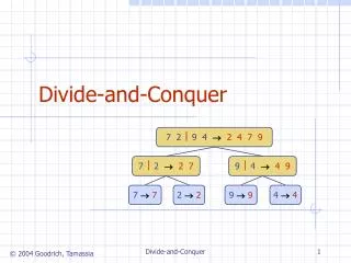
Merge Sort Approach • To sort an array A[p . . r]: • Divide • Divide the n-element sequence to be sorted into two subsequences of n/2 elements each • Conquer • Sort the subsequences recursively using merge sort • When the size of the sequences is 1 there is nothing more to do • Combine • Merge the two sorted subsequences
Merge Sort r p q Alg.: MERGE-SORT(A, p, r) if p < rCheck for base case then q ← (p + r)/2Divide MERGE-SORT(A, p, q)Conquer MERGE-SORT(A, q + 1, r) Conquer MERGE(A, p, q, r)Combine • Initial call:MERGE-SORT(A, 1, n) 1 2 3 4 5 6 7 8 5 2 4 7 1 3 2 6
1 2 3 4 5 6 7 8 q = 4 5 2 4 7 1 3 2 6 1 2 3 4 5 6 7 8 5 2 4 7 1 3 2 6 1 2 3 4 5 6 7 8 5 2 4 7 1 3 2 6 5 1 2 3 4 6 7 8 5 2 4 7 1 3 2 6 Example – n Power of 2 Divide
1 2 3 4 5 6 7 8 1 2 2 3 4 5 6 7 1 2 3 4 5 6 7 8 2 4 5 7 1 2 3 6 1 2 3 4 5 6 7 8 2 5 4 7 1 3 2 6 5 1 2 3 4 6 7 8 5 2 4 7 1 3 2 6 Example – n Power of 2 Conquer and Merge
1 2 3 4 5 6 7 8 9 10 11 q = 6 4 7 2 6 1 4 7 3 5 2 6 1 2 3 4 5 6 7 8 9 10 11 q = 3 4 7 2 6 1 4 7 3 5 2 6 q = 9 1 2 3 4 5 6 7 8 9 10 11 4 7 2 6 1 4 7 3 5 2 6 1 2 3 4 5 6 7 8 9 10 11 4 7 2 6 1 4 7 3 5 2 6 1 2 4 5 7 8 4 7 6 1 7 3 Example – n Not a Power of 2 Divide
1 2 3 4 5 6 7 8 9 10 11 1 2 2 3 4 4 5 6 6 7 7 1 2 3 4 5 6 7 8 9 10 11 1 2 4 4 6 7 2 3 5 6 7 1 2 3 4 5 6 7 8 9 10 11 2 4 7 1 4 6 3 5 7 2 6 1 2 3 4 5 6 7 8 9 10 11 4 7 2 1 6 4 3 7 5 2 6 1 2 4 5 7 8 4 7 6 1 7 3 Example – n Not a Power of 2 Conquer and Merge
r p q 1 2 3 4 5 6 7 8 2 4 5 7 1 2 3 6 Merging • Input: Array Aand indices p, q, rsuch that p ≤ q < r • Subarrays A[p . . q] and A[q + 1 . . r] are sorted • Output: One single sorted subarray A[p . . r]
r p q 1 2 3 4 5 6 7 8 2 4 5 7 1 2 3 6 Merging • Idea for merging: • Two piles of sorted cards • Choose the smaller of the two top cards • Remove it and place it in the output pile • Repeat the process until one pile is empty • Take the remaining input pile and place it face-down onto the output pile A1 A[p, q] A[p, r] A2 A[q+1, r]
p q r Example: MERGE(A, 9, 12, 16)
Example (cont.) Done!
p q 2 4 5 7 L q + 1 r r p q 1 2 3 6 R 1 2 3 4 5 6 7 8 2 4 5 7 1 2 3 6 n2 n1 Merge - Pseudocode Alg.:MERGE(A, p, q, r) • Compute n1and n2 • Copy the first n1 elements into L[1 . . n1 + 1] and the next n2 elements into R[1 . . n2 + 1] • L[n1 + 1] ← ;R[n2 + 1] ← • i ← 1; j ← 1 • for k ← pto r • do if L[ i ] ≤ R[ j ] • then A[k] ← L[ i ] • i ←i + 1 • else A[k] ← R[ j ] • j ← j + 1
Running Time of Merge(assume last for loop) • Initialization (copying into temporary arrays): • (n1 + n2) = (n) • Adding the elements to the final array: - n iterations, each taking constant time (n) • Total time for Merge: • (n)
Analyzing Divide-and Conquer Algorithms • The recurrence is based on the three steps of the paradigm: • T(n) – running time on a problem of size n • Divide the problem into a subproblems, each of size n/b: takes D(n) • Conquer (solve) the subproblems aT(n/b) • Combine the solutions C(n) (1) if n ≤ c T(n) = aT(n/b) + D(n) + C(n) otherwise
MERGE-SORT Running Time • Divide: • compute qas the average of pand r:D(n) = (1) • Conquer: • recursively solve 2 subproblems, each of size n/2 2T (n/2) • Combine: • MERGE on an n-element subarray takes (n) time C(n) = (n) (1) if n =1 T(n) = 2T(n/2) + (n) if n > 1
Solve the Recurrence T(n) = c if n = 1 2T(n/2) + cn if n > 1 Use Master’s Theorem: Compare n with f(n) = cn Case 2: T(n) = Θ(nlgn)
Merge Sort - Discussion • Running time insensitive of the input • Advantages: • Guaranteed to run in (nlgn) • Disadvantage • Requires extra space N
The Master Theorem • Theorem 4.1 • Let a 1 and b > 1be constants, let f(n) be a function, and Let T(n) be defined on nonnegative integers by the recurrence T(n) = aT(n/b) + f(n), where we can replace n/b by n/b or n/b. T(n) can be bounded asymptotically in three cases: • If f(n) = O(nlogba–) for some constant > 0, then T(n) = (nlogba). • If f(n) = (nlogba), then T(n) = (nlogbalg n). • If f(n) = (nlogba+) for some constant > 0, and if, for some constant c < 1 and all sufficiently large n, we have a·f(n/b) c f(n), then T(n) = (f(n)). We’ll return to recurrences as we need them…
≤ Quicksort A[p…q] A[q+1…r] • Sort an array A[p…r] • Divide • Partition the array A into 2 subarrays A[p..q] and A[q+1..r], such that each element of A[p..q] is smaller than or equal to each element in A[q+1..r] • Need to find index q to partition the array
≤ Quicksort A[p…q] A[q+1…r] • Conquer • Recursively sort A[p..q] and A[q+1..r] using Quicksort • Combine • Trivial: the arrays are sorted in place • No additional work is required to combine them • The entire array is now sorted
QUICKSORT Alg.: QUICKSORT(A, p, r) ifp < r thenq PARTITION(A, p, r) QUICKSORT (A, p, q) QUICKSORT (A, q+1, r) Initially: p=1, r=n Recurrence: PARTITION()) T(n) = T(q) + T(n – q) + f(n)
A[p…i] x x A[j…r] i j Partitioning the Array • Choosing PARTITION() • There are different ways to do this • Each has its own advantages/disadvantages • Hoare partition (see prob. 7-1, page 159) • Select a pivot element x around which to partition • Grows two regions A[p…i] x x A[j…r]
A[p…r] 3 3 5 3 5 3 3 3 3 3 3 3 2 2 2 2 2 2 6 1 1 6 6 6 4 4 4 4 4 4 6 1 6 1 1 1 5 5 3 5 3 5 7 7 7 7 7 7 i j i j i j i j A[p…q] A[q+1…r] i j j i Example pivot x=5
5 ap 3 2 6 4 1 3 7 ar A[p…q] A[q+1…r] ≤ A: j=q i Partitioning the Array Alg.PARTITION (A, p, r) • x A[p] • i p – 1 • j r + 1 • while TRUE • do repeatj j – 1 • untilA[j] ≤ x • dorepeati i + 1 • untilA[i] ≥ x • ifi < j • then exchange A[i] A[j] • elsereturnj r p A: i j Each element is visited once! Running time: (n) n = r – p + 1
Recurrence Alg.: QUICKSORT(A, p, r) ifp < r thenq PARTITION(A, p, r) QUICKSORT (A, p, q) QUICKSORT (A, q+1, r) Initially: p=1, r=n Recurrence: T(n) = T(q) + T(n – q) + n
n n 1 n - 1 n n - 1 1 n - 2 n - 2 n 1 n - 3 1 3 2 1 1 2 (n2) Worst Case Partitioning • Worst-case partitioning • One region has one element and the other has n – 1 elements • Maximally unbalanced • Recurrence: q=1 T(n) = T(1) + T(n – 1) + n, T(1) = (1) T(n) = T(n – 1) + n = When does the worst case happen?
Best Case Partitioning • Best-case partitioning • Partitioning produces two regions of size n/2 • Recurrence: q=n/2 T(n) = 2T(n/2) + (n) T(n) = (nlgn) (Master theorem)
Case Between Worst and Best • 9-to-1 proportional split Q(n) = Q(9n/10) + Q(n/10) + n
n n 1 n - 1 (n – 1)/2 + 1 (n – 1)/2 (n – 1)/2 (n – 1)/2 Performance of Quicksort • Average case • All permutations of the input numbers are equally likely • On a random input array, we will have a mix of well balanced and unbalanced splits • Good and bad splits are randomly distributed across throughout the tree partitioning cost: n = (n) combined partitioning cost: 2n-1 = (n) Alternate of a good and a bad split Nearly well balanced split • Running time of Quicksort when levels alternate between good and bad splits is O(nlgn)