Download
1 / 55
610 likes | 810 Views
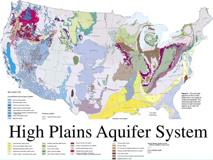
High Plains Aquifer System. Major rivers crossing the High Plains. Platte River. Arkansas River. Canadian River. Geologic History.

E N D
Major rivers crossing the High Plains Platte River Arkansas River Canadian River
Geologic History • Deposition of basement rocks, Permian-Tertiary. Permian contains evaporites, affect water quality, cause subsidence. Late Cretaceous seds contains gypsum. Doming centered on OK/TX • Laramide uplift in early Tertiary, seaway in midwest. • Large braided river system transport sed to the east off Rocky Mtns, Miocene to Pliocene. Coarse grn, variable sorting. Sand and gravel up to 1000 ft thick. Ogallala frm
Geologic History, Continued • Continued uplift tilts Ogallala frm. Removed by erosion near mountains, locally. • Dust storms deposit silt (loess) during Pleistocene, potential confining units • Eolian processes rework . Dunes formed. • Modern river systems rework. Alluvium formed
Basement geology • Cretaceous SS contribute water • Marine basement rocks affect water quality, Cl, SO4
Geologic units within the High Plains aquifer system • Alluvium • Dune sand • Ogallala Frm • Airkaree Frm • Brule Frm
Fence diagram Regional dip
Rule of Vs Dip of the lower contact relative to the gradient of dissecting rivers
Gaining reach, channel cut through HP to bedrock Fence diagram Losing reach, channel underlain by HP Regional dip
Basic Characteristics • Thick, unconfined aquifer. Locally confined by loess or caliche • K: 10 to 100 m/day; 30m/day average 30m/day = 3x10⁻⁴ m/s • b: 300 m max; 30 m average • T: 1000 m2/day • S: 0.1 to 0.3; 0.15 average (specific yield)
Recharge Ave Magnitude: increases from 1 mm/yr in N.TX to 150 mm in dunes in NE • Infiltration on uplands • Losing streams; ephemeral streams with permeable beds (1.3% loss/mile in one study). Locally streams losing due to pumping • Irrigation return (irrigation-ET) • Bedrock (where upward flow occurs) Factors affecting distribution of recharge…
How to estimate distributed recharge? One approach…. • Water balance on vadose zone Precipitation = ET + Interflow + Recharge Where interflow is small (low slope, far from drainage) Recharge = Precipitation – ET • Important factors Precipitation, Temp, Vegetation, Slope, K of surface materials
Potential ET Potential ET produced when rate is limited by energy input and plant metabolism, not limited by availability of water. Potential ET >Actual ET
Mean lake evaporation Figure 3. Mean annual lake evaporation in the conterminous United States, 1946-55. Data not available for Alaska, Hawaii, and Puerto Rico. (Source: Data from U.S. Department of Commerce, 1968).
Playa lake on High Plains aq in TX panhandle20,000 playa lakes in TX
Playas = important feature affecting recharge of High Plains aquifer • Focused recharge • Amount of recharge • Distribution • Water quality • Timing Uniformly distributed recharge
Discharge • Streams; perennial, ephemeral • Seeps, springs • Riparian ET. May be significant where w.t. shallow (near surface water) • Wells
What is the average horizontal hydraulic head gradient • What is the horizontal gw flux in the aquifer (m/d)? • What is the average gw velocity? (m/d) • Use the head contours to identify an area of suspected recharge. Circle the area, write “R” and draw gw flux vectors. List both geologic and meteorologic factors supporting your choice of recharge area • Identify an area of negligible recharge. List geologic or meteorologic factors supporting your choice of recharge area. Circle and write “NR” and draw gw flux vectors. • Identify a gaining stream reach. Circle and write “G” draw gw flux vectors • Identify a losing stream reach. Circle and write “L” and draw gw flux vectors
= 40 miles Hydraulic gradient 400 ft/40 miles 10 ft/mile =1/500 = 0.002 Flux: 0.002* 30 m/d = 0.06 m/day Velocity = 0.06/0.2 = 0.3 m/d Hydraulic head contours in High Plains aquifer
Gaining reach Losing reach Evidence for gw/sw interaction
Diverging flow Possibly recharge here R Parallel flow, uniform gradient Recharge? Evidence for recharge
Water Use • Pre-1930s: Irrigation from surface water. Dust Bowl Drought • 1930s Centrifugal well pump developed. • 1949: 2x10⁶ acres mostly N TX. Platte R. • 1950s-60s: Drought. Oil and gas=energy source, more irrigation • 1960s: Centrifugal pump improved. 750 gpm well = central pivot irrigation, r=0.25 mi • 1978: 27000 central pivot systems, 13x106 acres • Pumping exceeds recharge by 100+x • Water levels drop 100 ft+. GW mining. Pumping costs increase
Roughly 4 x10⁶ acre ft/yr in KS Translate to flux to improve understanding KS, 150x200 miles=30000 mi2 639 acres=1mi2 19x106 acres Or 4/19=0.2 ft/yr Roughly 4 x10⁶ acre ft/yr in KS Significance??
Figure 5. Irrigated cropland 1992, Northern Plains region. USDA, NRCS, Lambert Conformal Conic Projection, 1927 North American Datum. Source: National Cartography and GIS Center, NRCS, USDA, Ft. Worth, TX, in cooperation with the natural Resources Inventory Division, NRCS, USDA, Washington, D.C., using GRASS/MAPGEN software, 09/95. Map based on data generated by NRI Division using 1992 NRI. Because the statistical variance in some of these areas may be large, the map reader should use this map to identify broad trends and avoid making highly localized interpretations Irrigated land, 1992
Predevelopment to 1980 Aquifer sustainabilityWater balanceEco-impactChemistry Water balance on aquifer Recharge+Irrigation return = Baseflow + Pumping + Riparian ET + rate of change of storage
Water storage in aquiferPredevelopment saturated thickness in KS