Download

1 / 17
170 likes | 384 Views
Root Locus Plot of Dynamic Systems. imtiaz.hussain@faculty.muet.edu.pk. We will cover. Root Locus of LTI models Root locus of a Transfer Function (TF) model Root Locus of 1 st order system Root Locus of 2 nd order system Root Locus of higher order systems

E N D
Root Locus Plot of Dynamic Systems imtiaz.hussain@faculty.muet.edu.pk
We will cover........ • Root Locus of LTI models • Root locus of a Transfer Function (TF) model • Root Locus of 1st order system • Root Locus of 2nd order system • Root Locus of higher order systems • Root locus of a Zero-pole-gain model (ZPK) • Root locus of a State-Space model (SS) • Gain Adjustment
Root Locus of 1st Order System Consider the following unity feedback system Matlab Code num=1; den=[1 0]; G=tf(num,den); rlocus(G) sgrid
Root Locus of 1st Order System Consider the following unity feedback system num=[1 0]; den=[1 1]; G=tf(num,den); rlocus(G) sgrid Continued…..
Plot the root locus of following first order systems. Exercise#1
Root Locus 2nd order systems Consider the following unity feedback system num=1; den1=[1 0]; den2=[1 3]; den=conv(den1,den2); G=tf(num,den); rlocus(G) sgrid Determine the location of closed loop poles that will modify the damping ratio to 0.8 and natural undapmed frequency to 1.7r/sec. Also determine the gain K at that point.
Exercise#2 Plot the root locus of following 2nd order systems. (1) (2)
Root Locus of Higher Order Systems Consider the following unity feedback system num=1; den1=[1 0]; den2=[1 1]; den3=[1 2]; den12=conv(den1,den2); den=conv(den12,den3); G=tf(num,den); rlocus(G) sgrid Determine the closed loop gain that would make the system marginally stable.
Exercise#3 Plot the root locus of following systems. (1) (2)
Root Locus of a Zero-Pole-Gain Model k=2; z=-5; p=[0 -1 -2]; G=zpk(z,p,k); rlocus(G) sgrid
Root Locus of a State-Space Model A=[-5 -1;3 -1]; B=[1;0]; C=[1 0]; D=0; sys=ss(A,B,C,D); rlocus(sys) sgrid
Exercise#4: Plot the Root Locus for following LTI Models (1) (2) (3)
Choosing Desired Gain num=[2 3]; den=[3 4 1]; G=tf(num,den); [kd,poles]=rlocfind(G) sgrid
Exercise#5 (1) Plot the root Loci for the above ZPK model and find out the location of closed loop poles for =0.505 and n=8.04 r/sec. b=0.505; wn=8.04; sgrid(b, wn) axis equal
Exercise#5:(contd…) Consider the following unity feedback system (2) Plot the root Loci for the above transfer function Find the gain when both the roots are equal Also find the roots at that point Determine the settling of the system when two roots are equal.
Exercise#5:(contd…) Consider the following velocity feedback system (3) Plot the root Loci for the above system Determine the gain K at which the the system produces sustained oscillations with frequency 8 rad/sec.
End of tutorial You can download this tutorial from:http://imtiazhussainkalwar.weebly.com/