Download
1 / 117
1.39k likes | 2.39k Views
CHAPTER 4. The Laplace Transform. Chapter Contents. 4.1 Definition of the Laplace Transform 4.2 The Inverse Transform and Transforms of Derivatives 4.3 Translation Theorems 4.4 Additional Operational Properties 4.5 The Dirac Delta Function 4.6 Systems of Linear Differential Equations.

E N D
CHAPTER 4 The Laplace Transform
Chapter Contents • 4.1 Definition of the Laplace Transform • 4.2 The Inverse Transform and Transforms of Derivatives • 4.3 Translation Theorems • 4.4 Additional Operational Properties • 4.5 The Dirac Delta Function • 4.6 Systems of Linear Differential Equations
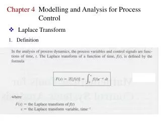
4.1 Definition of Laplace Transform • Basic DefinitionIf f(t)is defined for t 0,then(1) If f(t)is defined for t 0,then(2)is said to be the Laplace Transformof f. Definition 4.1.1 Laplace Transform
Example 1 Using Definition 4.1.1 Evaluate L {1} Solution:Here we keep that the bounds of integral are 0 and in mind.From the definitionSince e-st 0as t ,for s > 0.
Example 2 Using Definition 4.1.1 Evaluate L {t} Solution:
Example 3 Using Definition 4.1.1 Evaluate L {e-3t} Solution:
Example 4 Using Definition 4.1.1 Evaluate L {sin2t} Solution:
Example 4 (2) Laplace transform of sin 2t ↓
L is a Linear Tramsform • We can easily verify that(3)
Theorem 4.1.1 Transform of Some Basic Functions (a) (b) (c) (d) (e) (f) (g)
A function f(t)is said to be of exponential order, if there exists constants c, M > 0, and T > 0,such that |f(t)| Mect for all t > T. See Fig 4.1, 4.2. Definition 4.1.2 Exponential Order
Fig 4.1.3 Functions with blue graphs are of exponential order
Theorem 4.1.2 Sufficient Conditions for Existence If f(t) is piecewise continuous on [0, ) and of exponential order c, then L {f(t)}exists for s > c.
Example 5 Find L {f(t)}for Solution:
4.2 The Inverse Transform and Transform of Derivatives (a) (b) (c) (d) (e) (f) (g) Theorem 4.2.1 Some Inverse Transform
Example 1 Applying Theorem 4.2.1 Find the inverse transform of (a) (b) Solution:(a)(b)
L-1 is also linear • We can easily verify that(1)
Example 2 Termwise Division and Linearity Find Solution:(2)
Example 3 Partial Fractions and Linearity Find Solution:Using partial fractionsThen (3)If we set s = 1, 2, −4,then
Example 3 (2) (4)Thus (5)
Transform of Derivatives • (6) • (7) (8)
If are continuous on [0, ) and are of exponential order and if f(n)(t) is piecewise-continuous On [0, ), thenwhere Theorem 4.2.2 Transform of a Derivative
Solving Linear ODEs • Then(9)(10)
Example 4 Solving a First-Order IVP Solve Solution:(12)(13)
Example 4 (2) We can find A = 8, B = −2, C = 6Thus
Example 5 Solving a Second-Order IVP Solve Solution:(14)Thus
Theorem 4.3.1 First Translation Theorem If L {f} = F(s) and a is any real number, then L {eatf(t)} = F(s – a) 4.3 Translation Theorems Proof:L {eatf(t)} = e-steatf(t)dt = e-(s-a)tf(t)dt = F(s – a)
Example 1 Using the First Translation Theorem Evaluate (a) (b) Solution:(a)(b)
Inverse Form of Theorem 4.3.1 • (1)where
Example 2 Partial Fractions and Completing the square Evaluate (a) (b) Solution:(a) we have A = 2, B = 11(2)
Example 2 (2) And(3)From (3), we have(4)
Example 2 (3) (b) (5)(6)(7)
Example 3 IVP Solve Solution:
Example 3 (2) • (8)
Example 4 An IVP Solve Solution:
The Unit Step FunctionU (t – a)is Definition 4.3.1 Unit Step Function See Fig 4.3.2.
Also a function of the type(9)is the same as(10)Similarly, a function of the type(11)can be written as (12)
Example 5 A Piecewise-Defined Function Express in terms of U (t). Solution:From (9) and (10), with a = 5, g(t) =20t, h(t) = 0f(t) =20t – 20tU (t – 5) Consider the function (13)See Fig 4.3.5.