Download
1 / 58
580 likes | 804 Views
AOD Tutorial. These slides can be found in ppt in http://hepunx.rl.ac.uk/atlasuk/simulation/level2/egamma/tutorial/Tutorial_AOD_100305.ppt In pdf http://hepunx.rl.ac.uk/atlasuk/simulation/level2/egamma/tutorial/Tutorial_AOD_100305.pdf. AOD Tutorial. Outline Transferring files via DonQuixote

E N D
AOD Tutorial • These slides can be found in ppt in • http://hepunx.rl.ac.uk/atlasuk/simulation/level2/egamma/tutorial/Tutorial_AOD_100305.ppt • In pdf • http://hepunx.rl.ac.uk/atlasuk/simulation/level2/egamma/tutorial/Tutorial_AOD_100305.pdf M. Wielers, RAL
AOD Tutorial • Outline • Transferring files via DonQuixote • Exercise 1: • Copy a file via DonQuixote • Overview of ESD/AOD production • Interactive AOD session • Exercise 2: • Basic set-up • Exercise 3: • Look at AOD interactively • Exercise 4: • Basic set-up • retrieve electron container and plot some quantities • Useful tools four-momentum, particle, navigable • Exercise 5: • plot invariant Z-mass • Some more useful tools • Exercise 6: • Use some tools to plot Z-mass M. Wielers, RAL
Transferring files via DonQuixote • Most of ESD/AOD prod for Rome will be centrally produced via GRID • To find out about the Status of Rome productions and available samples • https://uimon.cern.ch/twiki/bin/view/Atlas/RomeStatusWiki • http://atlfarm003.mi.infn.it/%7Enegri/rome_dataset.htm • Files can be transferred via DonQuixote • https://uimon.cern.ch/twiki/bin/view/Atlas/RomeGetFilesWiki • What is it • ATLAS Experiment Data Management System • integrate all Grid data management services used by ATLAS • provide production managers and physicists access to file-resident event data • implementing data flow as defined by the ATLAS Computing Model • In short: mean to access “official” ATLAS data produced on the GRID • Documentation how to use it in • https://uimon.cern.ch/twiki/bin/view/Atlas/DonQuijoteEndUserClient • To transfer files you need a GRID certificate and be registered with ATLAS VO • You can install DonQuixote in your lab on a machine with GRID UI M. Wielers, RAL
Basic GRID set-up • At CERN lxplus can act as a GRID machine • To be able to run there we have to export the keys and get them on lxplus • This was the exercise to do prior to the tutorial. If you havn’t done so, follow the instructions and watch over someone else’s shoulder • http://www.grid-support.ac.uk/ca/user-documentation/uk-esc-documentation.pdf • http://msmizans.home.cern.ch/msmizans/production/dc2/grid0.html • To enable your lxplus session to act as UI • source /afs/cern.ch/project/gd/LCG-share/2.3.0/sl3/etc/ profile.d/grid_env.sh • source /afs/cern.ch/project/gd/LCG-share/2.3.0/rh73/etc/ profile.d/grid_env.sh • Obtain temporary grid proxy certificate • grid-proxy-init -valid Hours:Minutes • (if you don’t give the time, you’ll get 8h) • At the end of your session • grid-proxy-destroy M. Wielers, RAL
Export your key to CERN • Follow indications “how to export your key” in • http://www.grid-support.ac.uk/ca/user-documentation/uk-esc-documentation.pdf • Then let’s install it to CERN (instructions in web page out-dated, so let’s do it together) • http://msmizans.home.cern.ch/msmizans/production/dc2/grid0.html • Log on lxplus7 and in your home directory, do the following, assuming the key is called: MyKeys.pfx • source /afs/cern.ch/project/gd/LCG-share/2.3.0/rh73/etc/ profile.d/grid_env.sh • openssl pkcs12 -in MyKeys.pfx -clcerts -nokeys -out usercert.pem • openssl pkcs12 -in MyKeys.pfx -nocerts -out userkey.pem • chmod 400 userkey.pem • chmod 444 usercert.pem • mkdir .globus/ • mv *.pem .globus/ M. Wielers, RAL
How to use DonQuixote at CERN • Set up lxplus7 to act as GRID UI and identify yourself to the grid • Note: DonQuixote version 2 only works under RH7, version 3 about to come • source /afs/cern.ch/project/gd/LCG-share/2.3.0/rh73/etc/ profile.d/grid_env.sh • grid-proxy-init • The python script you need to use is installed at CERN • /afs/cern.ch/atlas/offline/external/DQClient/dms2/dms2.py • Basic commands you are likely to use are: • Search for a dataset • dms2.py search ‘rome.003025.digit.B4_jets17filter*’ • dms2.py search ‘rome.003025.digit.B4_jets17filter*’ > dijet.out (more convenient) • Copy data to castor (for LCG files) • dms2.py get ‘rome.003025.digit.B4_jets17filter._02010.pool.root’ -–remote • dms2.py get ‘rome.003025.digit.B4_jets17filter*’ --copy –-remote -–multiple • For files from grid3 or NorduGrid (ng) • dms2.py –g grid3 or dms2.py –g ng M. Wielers, RAL
Exercise 1: copy a file via Grid • Install your GRID key at CERN • Execute the grid-init • Ok, let’s try to see which files for dataset “rome.003025.digit.B4_jets17filter*’” was produced • Now copy one of the files to CERN • Note: in the CERN setup the datafile will automatically end up in the castor grid directory • /castor/cern.ch/grid/atlas/datafiles/<prod>/<type> • <prod> = dc1, dc2, rome • <type> = evgen, simul, digit, reco • Note: at the end of the copy there will be some error messages, however, the copy probably worked • Check you see it in the castor directory • Don Quixote is a bit buggy, so sometimes you have to try again, some datasets such as digitcalib doesn’t seem to be accepted by the tool. • Very likely we don’t have to worry for the large scale AOD Rome productions • The files will be available at CERN from a castor scratch area M. Wielers, RAL
Brief Overview of ESD/AOD production • ESD : Event Summary Data • Detailed output of reconstruction • Contains main reconstruction objects, such a EM clusters, track particles, muons, taus, jets… • Gives as well list of cells belonging to a cluster, space-points belonging to a track…. • Thus refinements of combined reco. e.g. particle id, track refitting, jet calibration possible • Things such as re-doing pattern recognition, re-calibration of cells not possible • AOD: Analysis Object Data • Only necessary information to perform most analysis available • data organised into analysis objects whose classes have physical meaning • Electron, photon, jet, tau, muon, … • Also TrackParticle • essential aspect is truth association, which directly links the original Monte Carlo data to the reconstructed objects • AOD is formed from the ESD through the use of AOD Builders • Back-navigation to ESD information possible M. Wielers, RAL
LVL1 calo variables, LVL2 calo + track variables M. Wielers, RAL
How to produce an ESD • Some pre-defined jobOptions available • get_files optRecExtoESD.py • OptRectoESD.py • doWriteESD = True # ESD persistency flag • DetDescrVersion = "Rome-Initial" # Detector description • EvtMax = 5 #number of Event to process • doCBNT = False # suppress ntuple • doHist = False # suppress histos • PoolRDOInput = ["rfio:/castor/cern.ch/xxxx/ MyAOD.pool.root" ] • # the input raw data file • PoolESDOutput = “ESD.pool.root” # output ESD name • To run • athena.py optRecExToESD.py ../share/RecExCommon_topOptions.py • Similar you can run together with the Trigger_forRecExCommon_jobOptions.py file from the TriggerRelease area and produce an ESD with offline and trigger information M. Wielers, RAL
How to produce an AOD • Some pre-defined jobOptions available • get_files optESDtoAOD.py • athena optESDtoAOD.py ../share/RecExCommon_topOptions.py • OptESDtoAOD.py • AllAlgs = False # Do not re-run the reco. • readESD = True # Read the ESD • doWriteAOD = True # AOD persistency output • DetDescrVersion = "Rome-Initial" # Detector description • doHist = False # suppress histograms • PoolESDInput = [ "ESD.pool.root" ] # ESD input file • PoolAODOutput = "AOD.pool.root“ # AOD output file • from AthenaCommon.DetFlags import DetFlags # Detector Flags • DetFlags.detdescr.ID_setOn() • DetFlags.detdescr.Calo_setOn() • DetFlags.detdescr.Muon_setOn() • # switch AOD streaming - we are not interested in that here • from ParticleEventAthenaPool.AODFlags import AODFlags • AODFlags.Streaming = False M. Wielers, RAL
How to produce an AOD • In addition something similar exists for ATLFAST • I don’t think we should try to do this here, but have a look at • http://www.usatlas.bnl.gov/PAT/tutorial904.html#Prod_ESD_AOD M. Wielers, RAL
Ok, let’s try to look at an AOD and do basic set-up • This tutorial is based on release 10 • Though AOD’s are from 9.0.4 • Not everything can be tested due to changes in persistified classes • E.g. back navigation doesn’t work • Let’s start with the basic set-up • Ask for Release 10.0.0 in cmt requirements file • source /afs/cern.ch/sw/contrib/CMT/v1r16p20040901/mgr/setup.sh • cmt config • source setup.sh –tag=opt • create Tutorial area (where ever it’s convenient) • cd to your tutorial area • cmt co -r UserAnalysis-00-02-00 PhysicsAnalysis/AnalysisCommon/UserAnalysis • cmt co Control/AthenaServices • cdPhysicsAnalysis/AnalysisCommon/UserAnalysis/ UserAnalysis-00-02-00/src • cp ~mwielers/maxidisk/tutorial_files/AnalysisSkeleton.cxx . • cd ../UserAnalysis M. Wielers, RAL
Exercise 2: Basic set-up for tutorial • cp ~mwielers/maxidisk/tutorial_files/AnalysisSkeleton.h . • cd ../cmt • Add AthenaServices to your requirements • Use AthenaServices AthenaServices-* Control • cmt bro cmt config • source setup.sh • cmt bro gmake • cd ../run • cp ~mwielers/maxidisk/tutorial_files/PoolFileCatalog.xml . • get_files PDGTABLE.MeV • cp ~mwielers/maxidisk/tutorial_files/AnalysisSkeleton_jobOptions.py . • cp ~mwielers/maxidisk/tutorial_files/zee.aod.py . • Let’s look at an ESD and AOD by just opening the pool file and see what persistified object are in there • Open ESD file with root • ~mwielers/maxidisk/tutorial_files/ESD.pool.root • Do you see some trigger stuff? • Open AOD file with root • ~mwielers/maxidisk/tutorial_files/AOD.pool.root M. Wielers, RAL
Interactive AOD session • Unfortunately it only works under RH73 and doesn’t run out of the box in 10 • cmt co Control/AthenaServices (already done) • Only works on AOD’s not directly on ESD’s (though possible via back-navigation) • get_files -jo Interactive_topO.py • pool_insertFileToCatalog /afs/cern.ch/user/m/mwielers/maxidisk/tutorial_files/AOD.pool.root • edit the jobO (if needed) • e.g., change input file • EventSelector.InputCollections = [ "AOD.pool.root" ] • To • EventSelector.InputCollections = [ “/afs/cern.ch/user/m/mwielers/maxidisk/tutorial_files/AOD.pool.root" ] • Or • EventSelector.InputCollections = [ “rfio/castor/cern.ch/user/m/mwielers/aod/AOD.pool.root" ] • EventSelector.InputCollections = • ["AOD.pool_1.root“, “AOD.pool_2.root”] M. Wielers, RAL
start an interactive session • athena -i Interactive_topO.py -l FATAL • Don’t forget -i option!! • MCTruth::TruthStrategyManager: registered strategy DMuonCatchAll • MCTruth::TruthStrategyManager: registered strategy IDETIonization • MCTruth::TruthStrategyManager: registered strategy IDETDecay • MCTruth::TruthStrategyManager: registered strategy IDETConversion • MCTruth::TruthStrategyManager: registered strategy IDETBrems • MCTruth::TruthStrategyManager: registered strategy CALOCatchAll • ==> New TileCablingService created • Loaded dictionary PyAnalysisCoreDict • Loaded dictionary PyParticleToolsDict • Loaded dictionary PyTriggerToolsDict • Loaded dictionary PyKernelDict • Initialize application manager • athena> theApp.initialize() • Run 1 event • athena> theApp.nextEvent() M. Wielers, RAL
Basic commands in interactive AOD session • Retrieve ElectronCollection • athena> econ = PyParticleTools.getElectrons("ElectronCollection") • where “ElectronCollection” is key name in the StoreGate. Other methods are defined in PyParticleTools e.g., for Muon, PyParticleTools.getMuons(”MuonCollection”) • Number of electrons • athena> len(econ) • 5 • Get the first electron • athena> e = econ[0] • See pT • athena> e.pt() • 33299.1563339692 • Create and fill a ROOT histogram on the fly: • plot("ElectronContainer#ElectronCollection","$x.pt()",nEvent=5) • nEvent has to be less than the number of events in the file… • Only works once, then you’re at the end of the file and we don’t know how to re-start, unless you re-start your interactive session M. Wielers, RAL
Get a list of methods • athena> dir(e) • ['Electron', 'Navigable', 'P4EEtaPhiM', '_C_instance', '_C_metaclass', '__class__', '__del__', '__delattr__', '__dict__', '__doc__', '__getattribute__', '__hash__', '__init__', '__module__', '__new__', '__reduce__', '__reduce_ex__', '__repr__', '__setattr__', '__str__', '__weakref__', '_empty_instance', '_made_in_Python', 'author', 'begin', 'charge', 'contains', 'cosTh', 'cotTh', 'd0wrtPrimVtx', 'dataType', 'e', 'eg', 'end', 'et', 'eta', 'fillToken', 'getContainer', 'getEgammaWeight', 'getIndex', 'getParameter', 'hasCharge', 'hasPdgId', 'hasTrack', 'hlv', 'iPt', 'isEM', 'm', 'm_author', 'm_charge', 'm_constituents', 'm_dataType', 'm_e', 'm_eta', 'm_hasCharge', 'm_hasPdgId', 'm_hasTrack', 'm_isEM', 'm_m', 'm_origin', 'm_parameters', 'm_pdgId', 'm_phi', 'm_track', 'numberOfBLayerHits', 'numberOfPixelHits', 'numberOfSCTHits', 'numberOfTRTHighThresholdHits', 'numberOfTRTHits', 'origin', 'p', 'parameter', 'pdgId', 'phi', 'pt', 'putElement', 'px', 'py', 'pz', 'remove', 'removeAll', 'set4Mom', 'setE', 'setEta', 'setM', 'setPhi', 'set_all', 'set_charge', 'set_dataType', 'set_eg', 'set_isEM', 'set_origin', 'set_parameter', 'set_pdgId', 'set_track', 'sinTh', 'size', 'track', 'z0wrtPrimVtx', '~Electron', '~I4Momentum', '~INavigable', '~INavigable4Momentum', '~IParticle', '~Navigable', '~P4EEtaPhiM', '~P4EEtaPhiMBase', '~ParticleBase'] • Unfortunately you don’t just see the members, but as well all method provided by the class M. Wielers, RAL
See AOD contents using PyPoolBrowser • athena> include ("PyAnalysisExamples/PyPoolBrowser.py") • double-click “/” • click “+” of ElectronCollection → “+” on 0 → double click on “pt”, then you will see a histogram for pT distribution of electrons • Doesn’t really work in 9.0.4 • Be patient… very slow • Unfortunately only works on AOD’s right now, not on ESD’s • Use Ctrl-D to exit M. Wielers, RAL
Exercise 2: Interactive AOD session • Do basic set-up • Run interactive AOD session and try out some of the commands • For more examples/possibilities, see • http://tmaeno.home.cern.ch/tmaeno/Inter.htm • Allows navigation via ElementLink • going from electron track track quantities • Allows navigation back to ESD • e.g. electron egammaObject in ESD M. Wielers, RAL
How to access the Container • Just as you do in the reconstruction • Retrieve via StoreGate • Example: • std::string m_electronContainerName = "ElectronCollection"; • ... • const ElectronContainer* elecTES; • sc=m_storeGate->retrieve( elecTES, m_electronContainerName ); • if( sc.isFailure() || !elecTES ) { • mLog << MSG::WARNING << "No AOD electron container" << endreq; • return StatusCode::SUCCESS; } • mLog << MSG::DEBUG << "ElectronContainer retrieved" << endreq; • ... • // iterators over the container • ElectronContainer::const_iterator elecItr = elecTES->begin(); ElectronContainer::const_iterator elecItrE = elecTES->end(); • for (; elecItr != elecItrE; ++elecItr) { • double pT = (*elecItr)->pt(); • ... M. Wielers, RAL
StoreGate keys for AOD Container (1) M. Wielers, RAL
StoreGate keys for AOD Container (2) M. Wielers, RAL
StoreGate keys for Atlfast AOD Container M. Wielers, RAL
Glimpse at one of the classes: Electron • Electron.h in PhysicsAnalysis/AnalysisCommon/ParticleEvent • class Electron : public ParticleBase, • public P4EEtaPhiM, • public Navigable<egammaContainer,double> { • int isEM() const { return m_isEM; } • bool hasTrack() const { return m_hasTrack; } • const Rec::TrackParticle* track() const • { return ((m_hasTrack) ? (*m_track) : 0) ; } • Via navigation to track (e.g. (*m_track)->trackSummary()->get( Trk::numberOfBLayerHits ) ) • double z0wrtPrimVtx() const ; • double d0wrtPrimVtx() const ; • int numberOfBLayerHits() const • int numberOfPixelHits() const; • int numberOfSCTHits() const; • int numberOfTRTHits() const; • int numberOfTRTHighThresholdHits() const; M. Wielers, RAL
ElectronParamDefs.h enum ParamDef { // common enums EoverP = 0, // Enum's for egamma etaBE2 = 1, et37 = 2, e237 = 3, e277 = 4, ethad1 = 5, weta1 = 6, weta2 = 7, f1 = 8, e2tsts1 = 9, emins1 = 10, wtots1 = 11, fracs1 = 12, epiNN = 13, // Enum's for softe etaCorrMag = 1, f1core = 2, f3core = 3, Pos7 = 4, Iso = 5, Widths2 = 6, emWeight = 7, pionWeight = 8 Glimpse at one of the classes: Electron Access via • (*elec)->parameter(ElectronParameters::EoverP) M. Wielers, RAL
To find out which objects in each class • Hopefully soon via PAT web page • https://uimon.cern.ch/twiki/bin/view/Atlas/PhysicsAnalysisTools • At least that’s promised for in the next weeks • Via interactive python session • Unfortunately you get more than just the class members, also all methods • But probably the easiest way right now • Via doxigen • Look directly at class in release area • Some members in Kyle’s talk • http://agenda.cern.ch/fullAgenda.php?ida=a045107#s2 • Ask an “expert” M. Wielers, RAL
More about 4-momentum • Most particles such as electrons, photons, muon, tau, jets inherit from I4Momentum • For example: • for (; elecItr != elecItrE; ++elecItr) { • if( (*elecItr)->pt()> m_etElecCut ) { • double electronEta = (*elecItr)->eta(); • ... • Complete list • double px(), py(), pz(), m() • double p(), eta(), phi() • double e(), et(), pt(), double iPt() • double cosTh(), sinTh(), cotTh() • HepLorentzVector hlv() M. Wielers, RAL
HepLorentzVector • xxx M. Wielers, RAL
Exercise 4 • Modify AnalysisSkeleton.cxx and plot some histograms of quantities in the ElectronContainer • Retrieve ElectronContainer • Plot size of it • Plot pT, eta and EoverP of the electron candidates with pT>20GeV • Run and check your histograms with root • Watch out for the fix me in the code! M. Wielers, RAL
More about Particle • Particle have a 4-momentum representation (see more on next slide) • Particles have constituents (e.g. are navigable) • Daughters from particle decay • Reconstruction-level object • methods of IParticle M. Wielers, RAL
in Event/EventKernel M. Wielers, RAL
Navigation • Navigation to Constituents from AOD back to ESD: • CompositeParticle* W = new CompositeParticle(); • W->add(jetContainer, jet1, jet2); • If (!W->contains(jet3)) { do something;} • NavigationToken<CaloCell,double>* cellToken = new NavigationToken<CaloCell,double>(); • jet->fillToken(*cellToken); • NavigationToken<CaloCell, double>::const_iterator c = cellToken->begin(); • NavigationToken<CaloCell,double>::const_iterator cend = cellToken->end(); • for(; c != cend; ++c) { • const CaloCell* thisCell = *c; • double weight = jet->getParameter(thisCell); // • double weight = (*c).second; • double et = weight * thisCell->et(); • …. M. Wielers, RAL
Exercise 5: Plot inv. Z-mass • Add to AnalysisSkeleton.cxx • Use 4-vector method to combine 2 electrons with pT>20GeV and put it in histo • Run and check histo M. Wielers, RAL
Analysis Tools, Utilities • The following tools are currently available – • Look in CVS: • offline/PhysicsAnalysis/AnalysisCommon/ • AnalysisUtils • AnalysisTools • Main tools • Combination • Permutation • DeltaR matching • Selector • Filter • Special Utilities • Navigation • Association M. Wielers, RAL
IAnalysisTools • Delta phi between two particles • deltaPhi (const INavigable4Momentum *p1, const INavigable4Momentum *p2) • Delta R between 2 particles • double deltaR (const INavigable4Momentum *p1, const INavigable4Momentum *p2) • Invariant mass between 2 particles • imass2 (const INavigable4Momentum *p1, const INavigable4Momentum *p2) • Invariant mass between 4 particles • imass4 (const INavigable4Momentum *p1, const INavigable4Momentum *p2, const INavigable4Momentum *p3, const INavigable4Momentum *p4) M. Wielers, RAL
IAnalysisTools • find the closest (in R) element in a collection to an INavigable4Momentum • bool matchR (const INavigable4Momentum *t, COLL *coll, int &index, double &deltaR) • bool matchR (const INavigable4Momentum *t, COLL *coll, ELEMENT *element, double &deltaR) • bool matchR (const INavigable4Momentum *t, COLL *coll, int &index, double &deltaR, const int pdg) • sort by pT, eta, phi • sortPT (COLL *coll) • sortEta (COLL *coll) • sortPhi (COLL *coll) • classify by charge (pos, neg) • classifyCharge (const COLL *coll, std::vector<typename COLL::value_type> &pos, std::vector<typename COLL::value_type> &neg) M. Wielers, RAL
DeltaR Matching • Get a handle on the tools in the initialize() method: • IAlgTool *tmp_analysisTools; • sc = toolSvc->retrieveTool("AnalysisTools",tmp_analysisTools); • if (StatusCode::SUCCESS != sc) { • mLog << MSG::ERROR << "Can't get handle on ana tools" << endreq; • return StatusCode::FAILURE; } • Then in execute • m_analysisTools=dynamic_cast<IAnalysisTools *>(tmp_analysisTools); • int index = -1; • double deltaRMatch; • /// find a match to this electron in the MC truth container • /// the index and deltaR are returned • bool findAMatch = m_analysisTools->matchR((*elecItr), mcpartTES, index, deltaRMatch, (*elecItr)->pdgId()); • /// the matched object and deltaR are returned • bool findAMatch = m_analysisTools->matchR((*elecItr), mcpartTES, element, deltaRMatch, (*elecItr)->pdgId()); M. Wielers, RAL
Combination Example: Wjj • AnalysisUtils::Combination<const ParticleJetContainer> comb(jetTDS,2); • get all the combinations of 2 jets • std::vector<const IParticleContainer::base_value_type*> jj; • while (comb.get(jj)) { • double mjj = (jj[0]->hlv()+jj[1]->hlv()).m(); • m_jj->fill(mjj,m_eventWeight); • if ( fabs(mjj-mW) < m_deltaMjj ) { • CompositeParticle * Wjj = new CompositeParticle(); • Jet* newJet = new Jet( oldjet ) • Wjj->add(jetTDS,jj[0],jj[1]); • Wjj->set_charge(1); • Wjj->set_pdgId(PDG::W_plus); • Wjj->set_dataType(m_dataType); • m_WjjContainer->push_back(Wjj); } } } M. Wielers, RAL
Special Utility for Neutrino • In some analyses, you want to reconstruct neutrino • NeutrinoIParticle • To help you in PhysicsAnalysis/AnalysisCommon/SpecialUtils • candidatesFromWMass(lepton, pxMiss, pyMiss, neutrinoContainer) • neutrinosFromColinearApproximation(particleA, particleB, pxMiss, pyMiss, neutrinoContainer) • Objective is: each user does not have to write the same piece of code for general solutions to a subclass of problem • Example: use the W mass constraint for the pz solution of the neutrino momentum • for (; leptonItr != leptonItrE; ++leptonItr) { bool findNeutrino = NeutrinoUtils::candidatesFromWMass((*leptonItr), m_pxMiss, m_pyMiss, (*m_neutrinoContainer)); if (findNeutrino) { do something …} } M. Wielers, RAL
Special Particle: CompositeParticle • CompositeParticle is made up of other IParticles • add two particles to make a composite particle • In 9.0.4 (need symlink with ParticleBaseContainer) • CompositeParticle* myZ = new CompositeParticle • myZ->add(myBJetContainer, oldEle ) • In 10.0.0 (no need for container, but need to make a copy before adding) • CompositeParticle* myZ = new CompositeParticle • Electron* newEle = new Electron( oldEle ) • Composite particles can Navigate to its daughters M. Wielers, RAL
Creating Your Own Containers • MuonContainer * muonContainer = new MuonContainer(); • Muon * newMuon = new Muon(); • newMuonset_IDTrack(…); • newMuonset4Mom(HepLorentzVector(px,py,pz,e)); • … • muonContainer->push_back(newMuon); • m_storeGaterecord(muonContainer, “containerName”); • The muonContainer “owns” all the newMuon inside it: • Delete muonContainer; will also delete all the newMuon M. Wielers, RAL
Some caveats if you put particles in your container • PhotonContainer* photonContainer= new PhotonContainer(SG::VIEW_ELEMENTS); • photonContainerpush_back(newPhoton); • photonContainer does not own the newPhoton inside it • Delete photonContainer; will NOT delete the newPhotons • The AOD container that you retrieve from POOL owns its AOD • If you create your own container of pre-selected AOD, be careful: • m_userElectronContainer->push_back(*elecItr); • *elecItr is pointer to an Electron AOD in original electron AOD container: that container own *elecItr: m_userElectronContainer can NOT own *elecItr. So m_userElectronContainer must be previously created with “View elements” • Container ownership: SG::OWN_ELEMENTS, SG::VIEW_ELEMENTS M. Wielers, RAL
Exercise 6: again Z mass peak • This time use some of the tools you just learned • 1) Use tool for combinatorics • 2) Now write a selector which only selects electron with pT>20GeV and use that within the combinatorics tool • Note there is the method • bool goodOnes(CALLER *caller, OUT &comb, CRITERIA criteria) • with CALLER = AnalysisSkeleton • OUT = std::vector<const Electron*, std::allocator<const Electron*> > • CRITERIA = bool (AnalysisSkeleton::*) (const std::vector<const Electron*, std::allocator<const Electron*> >&), COLL = const ElectronContainer] • Selection routine must be friend of AnalysisSkeleton • You need something like • selectElectron(AnalysisSkeleton * self, const std::vector<const ElectronContainer::base_value_type*> &ll) M. Wielers, RAL