Download
1 / 27
280 likes | 394 Views
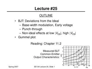
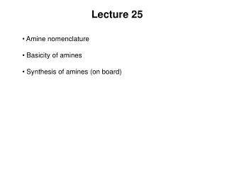
Lecture 25. Two-Phase Simple Upper Bounded Simplex Algorithm Example: Minimize –2x 1 – x 2 Subject to x 1 + x 2 < 6 0 < x 1 < 5 0 < x 2 < 5. The Graph. x 2 bound. x 2. x 1 bound. optimum. x 1. Convert To An Equality Constraint. Minimize –2x 1 – x 2

E N D
Lecture 25 • Two-Phase Simple Upper Bounded Simplex Algorithm • Example: • Minimize –2x1 – x2 • Subject to x1 + x2< 6 • 0 < x1< 5 • 0 < x2< 5
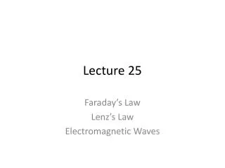
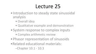
The Graph x2 bound x2 x1 bound optimum x1
Convert To An Equality Constraint • Minimize –2x1 – x2 • Subject to x1 + x2 +x3 = 6 • 0 < x1< 5 • 0 < x2< 5 • 0 < x3< Note Bound on the slack variable
Add An Artificial Variable • Minimize –2x1 – x2 • Subject to x1 + x2 +x3 + A= 6 • 0 < x1< 5 • 0 < x2< 5 • 0 < x3< • 0 < A <
Phase I Problem • Minimize A • Subject to x1 + x2 +x3 + A= 6 • 0 < x1< 5 • 0 < x2< 5 • 0 < x3< • 0 < A <
Step 0. Initialization • BASIC = {A at 6} • NONBASIC = {x1 at 0, x2 at 0, x3 at 0} • B = 1 • B-1 = 1
Step 1. Pricing • v = cBB-1 = 1(1) = 1 • cbar1 = c1 – va1 = 0 – 1(1) = -1 • cbar2 = c2 – va2 = 0 – 1(1) = -1 • cbar3 = c3 – va3 = 0 – 1(1) = -1 • All price favorably!
Step 2. Optimality • Not optimal • Let p = 3 - that is x3 is allowed to increase from 0
Step 3. Direction • y = B-1a3 = 1(1) = 1 • = 1 Why?
Step 4 Step Size • - = min{, (xj-ℓj)/(yj) : yj > 0} • + = min{, (uj-xj)/(-yj) : yj < 0} • = min{- , + , up - ℓp} • - = min{, (6-0)/1} = 6 • + = min{} = • = min{6, , -0} = 6
Step 5. New Point • XB = xB - y = 6 – 6(1)(1) = 0 • A = 0 • xp = x3 = ℓ3 + = 0 + 6 = 6 • Current Point: [x1,x2,x3,A] = [0,0,6,0] • BASIC = {x3 at 6} • NONBASIC = {x1 at 0, x2 at 0, A at 0} • B = 1 B-1 = 1
Step 1. Pricing • v = cBB-1 = 0(1) = 0 • cbar1 = c1 – va1 = 0 – 0(1) = 0 • cbar2 = c2 – va2 = 0 – 0(1) = 0 • All price unfavorably!
Step 2. Optimality • Optimal For Phase I
Phase II Problem • Minimize -2x1 – x2 • Subject to x1 + x2 +x3 = 6 • 0 < x1< 5 • 0 < x2< 5 • 0 < x3<
Step 1. Pricing • Current Point: [x1,x2,x3] = [0,0,6] • BASIC = {x3 at 6} • NONBASIC = {x1 at 0, x2 at 0} • B = 1 B-1 = 1 • v = cBB-1 = 0(1) = 0 • cbar1 = c1 – va1 = -2 – 0(1) = -2 • cbar2 = c2 – va2 = -1 – 0(1) = -1 • All price favorably!
Step 2. Optimality • Not Optimal • Let p = 1
Step 3. Direction • y = B-1a1 = 1(1) = 1 • = 1 Why?
Step 4 Step Size • - = min{, (xj-ℓj)/(yj) : yj > 0} • + = min{, (uj-xj)/(-yj) : yj < 0} • = min{- , + , up - ℓp} • - = min{, (6-0)/1} = 6 • + = min{} = • = min{6, , 5-0} = 5
Step 5. New Point • XB = xB - y = 6 – 5(1)(1) = 1 • x3 = 1 • xp = x1 = ℓ1 + = 0 + 5 = 5 • Current Point: [x1,x2,x3] = [5,0,1] • BASIC = {x3 at 1} • NONBASIC = {x1 at 5, x2 at 0} • B = 1 B-1 = 1 Note: The basis stayed the same.
Step 1. Pricing • v = cBB-1 = 0(1) = 0 • cbar1 = c1 – va1 = -2 – 0(1) = -2 Unfavorable Why? • cbar2 = c2 – va2 = -1 – 0(1) = -1 Favorable
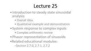
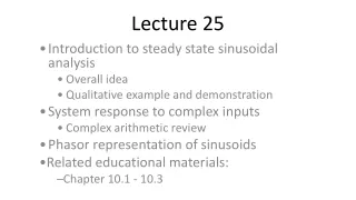
The Graph x2 bound x2 x1 bound current point x1
Step 2. Optimality • Not Optimal • Let p = 2
Step 3. Direction • y = B-1a1 = 1(1) = 1 • = 1 Why?
Step 4 Step Size • - = min{, (xj-ℓj)/(yj) : yj > 0} • + = min{, (uj-xj)/(-yj) : yj < 0} • = min{- , + , up - ℓp} • - = min{, (1-0)/1} = 1 • + = min{} = • = min{1, , 5-0} = 1
Step 5. New Point • XB = xB - y = 1 – 1(1)(1) = 0 • x3 = 0 • xp = x2 = ℓ2 + = 0 + 1 = 1 • Current Point: [x1,x2,x3] = [5,1,0] • BASIC = {x2 at 1} • NONBASIC = {x1 at 5, x3 at 0} • B = 1 B-1 = 1
Step 1. Pricing • v = cBB-1 = -1(1) = -1 • cbar1 = c1 – va1 = -2 – (-1)(1) = -1 Unfavorable Why? • cbar3 = c3 – va3 = 0 – (-1)(1) = 1 Unfavorable Why? • Optimality Obtained
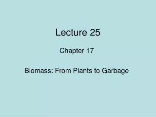
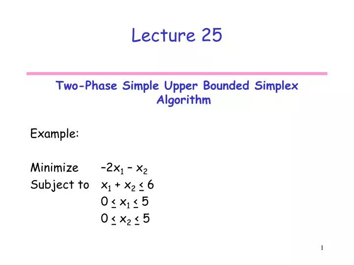
The Graph x2 bound x2 x1 bound current point x1