Download
1 / 45
450 likes | 555 Views
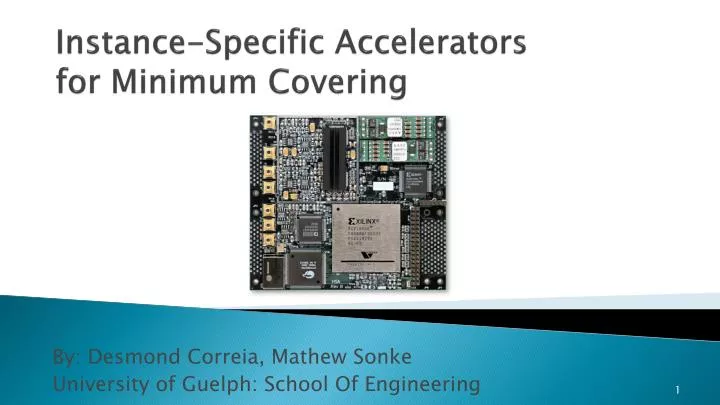
Instance-Specific Accelerators for Minimum Covering. By: Desmond Correia, Mathew Sonke University of Guelph: School Of Engineering. Outline. Background Information What is Instance Specific Hardware The Problem Solving the problem Hardware Approach Accelerator Architectures

E N D
Instance-Specific Accelerators for Minimum Covering By: Desmond Correia, Mathew Sonke University of Guelph: School Of Engineering
Outline • Background Information • What is Instance Specific Hardware • The Problem • Solving the problem • Hardware Approach • Accelerator Architectures • State Machines • Adapting to other problems • Experimentation • Simulation • Implementation • Discussion • Conclusion
What is Instance Specific Hardware • Hardware generates on the fly • Optimized for Algorithm • Optimized for Input Data • Formally • Generates circuit on the fly that depend on the problem instances rather than the problem • Useful when there is: • Need for fine-grained operators • Lots of parallelism • Long software run time
Instance Specific Hardware • Shaded blocks denote steps that are part of the accelerator’s runtime • Dynamically Compiles • Dynamically Configures • New problem = New hardware
What’s The Problem? • Boolean Satisfiability Problem (SAT) • Given a Boolean formula, find a variable assignment that equate it to 1 • F = (a + b)(a’ + b’ + c) = 1. One Solution: a = 1, c = 1 • Must be in Conjunctive Normal Form (CNF) • Minimum-Cost Covering Problem • Given a Universal Set: U = {1,2,3,4,5} • Given a set of subsets: S = { {1,2,3}, {2,4}, {3,4}, {4,5} } • Find smallest subset that contains all elements of U • T = { {1,2,3}, {4,5} }
Minimum-Cost Covering Problem • Try to cover a,b,c,d,e • Best Cover • S2, S4, S5 • Cost = 0.2+0.1+0.2 = 0.5
Why is the Problem Important? • Traveling Salesman problem • Shortest route to visit all the cities
Additional Applications • Scheduling of Airline crews • 2 level - Logic Synthesis • Have a set of minterms F(A,B,C,E) = ∑ m(0,2,7,10,11) • What is the optimal circuit for this? • Becomes a covering problem in order to generate an optimal Boolean function • Placement and Routing in FPGA • Decide location of each block while trying to minimize total length of interconnection
Matching Problem To Hardware • SAT problem Combinatorial problem • NP complete (Nondeterministic polynomial time) • Cannot be completed in polynomial time • Combinatorial problems exhibit • lots of parallelism • Often have very long runtimes • Requires fine-grained operators (XORing, ANDing, etc.). • Instance specific accelerators perfect for this
The Goal • Paper targets discrete optimization problem • Concentrate on exact solvers for minimum-cost covering problem • Global optimum solution • Minimum cost covering problem regarded as minimum cost SAT problem • Find a satisfying solution for a CNF that minimizes a linear cost function over the variables. • Paper published in 2003 in The Journal of Supercomputing
Solving The Problem • A = Matrix • V = current variable • B = current lowest cost solution • Iteratively reduce the matrix • Remove Essential Rows • Remove Dominating Columns • Remove Dominated Rows
Solve The Problem • No more reductions • Need to Compute cost bound • cost(v) + cost(minimum number of rows required to cover remaining columns) • Branch if cost of v ≤ b AND rows exist • Select variable • Assign it 1 and 0 • Both cases matrix is modified and algorithm is called recursively
Accelerator Architectures • State Machines: SM1… SMn • Control variable values • Implement one search level of branch and bound algorithm • SM connected to immediate neighbour • Branching to next SM • Backtrack to pervious SM • Output of SM: Current variable values
Accelerator Architectures • Checkers • Deduce information for partial variable assignment • Help us to figure out if to back track or continue • CNF Checkers • Don’t care Checker • Essential Checker • Dominated column Checker • All run in parallel
Accelerator Architectures • Cost Counter • Computes cost of current partial assignment • Controller • Initializes search procedure • Stops search procedure • Compute the cost bound
Backtracking with 3-valued Logic • Model to help with branching and backtracking • Three values: {0, 1, X} • X denoting unassigned variable • Allows for analyzing of partial assignment • Uses 3-valued logic to model • The Clause (a + b) (a’ + b’ + c) • The variable a, b, c • The CNF F = (a + b)(a’ + b’ + c)
Backtracking with 3-valued Logic. How it works? • All variable areinitially X • After value assignment CNF checker inspects results • CNF is 0: Backtrack i.e. NOT satisfiable (SAT) • CNF is 1: Valid cover found • If the cover is the least cost then save the variable assignment • Both cases: CNF=0 OR CNF=1 • Backtracking occurs to continue search on another path • Exploring of solution space
Backtracking with 3-valued LogicHow it works? • CNF is X: Continue searching on current path • Depending on: Checkers and cost bound results • Continues search with different value • State machine changes its assignment • Continue search by branching • Trigger next State machine • Backtrack • trigger previous state machine
CNF (Conjunctive Normal Form) Checker • Input vector: Current variable assignment • Clauses evaluated individually • (a + b) (a’ + b’ + c) • Results are ANDed together • Output: Single 3-valued logic signal • {1, 0, X }
Reductions Techniques • Reduction Checkers • Don’t cares • Essential Columns • Dominated Columns • Outputs: 2-valued Boolean logic • Implemented in pure combinatorial logic • Derived from CNF at compile time Function of Current variable Assignment
Don’t Care • Shares hardware with CNF Checker • CNF Checker computed 3-value logic • Only uses logic for {1, 0} • Variable set to ‘0’ indicates don’t care • Don’t care are derived from the clauses and covering matrix Shared CNF Checker
Essential Columns Checker • Generates essential condition for each variable • To make V4 essential • Set V3 = 0 • Reason • Only way to cover e4 WHEN V3 = 0
Dominated Column Checker • Variable corresponding to dominated column is set to ‘0’ • Module implements logic for each variable • Indicating the dominated condition • Evaluated when the state machine for the variable is activated • Only work on that column when covered by that variable • NOTE: Column is referring to a row in matrix presented before
Cost Counter • Approach • Algorithm implements unit cost; every variable has a cost of 0 or 1 • A new cost bound must be computed after every single variable assignment • Implementation • n-bit parallel counter • Adder that sums up n single bit inputs • Leverages Fast Carry Chain routing • n input bits results in l=log2(n) levels • Time delay Tctr=(l (l+1)/2)*Tadder
Cost Bound • Very simple implementation • Cost bound = current_best_cost – 1 • No estimation of cost by variables not yet searched
State Machines • Linear array of identical State Machines • Connections • From Top and To Top • From Below and To Below • Set 0 (Don’t care or Dominated Column) • Set 1 (Essential) • CNF Flag (1 or X) • Cost Exceeded Flag
State Machines Assign X If FT and not ST0 Assign 1 If CNF = X and not CEX TB If FB Assign 0 If CNF = X and not CEX TB If FB Assign X, TT (Backtrack) Else Backtrack Else Backtrack Else If FT and ST0 Assign 0 TB If FB Backtrack
Adapting to Other Problems • Reduction • Encapsulated into checker modules • Cost Bound • Encapsulated into controller module • Cost Counter • Unit cost can be replaced with integer cost by replacing Cost Counter with Cost Adder module
Testbench • Problems contained in DIMACS CNF file format • Code Generation • Perl program generates VHDL for each problem • VHDL code templates used for generic parts • Augmented with generated code for instance specific parts • Tools • Synopsys FPGA Compiler II • Xilinx 4.1i backend
Testbench • Problems • 16 small and 5 medium-sized problems from ESPRESSO-EXACT distribution • Problems have between 4 and 62 variables, and 4 to 70 clauses • Benchmarking • ESPRESSO-EXACT configured to output Cyclic Cores • Gives us the covering matrices just before first branch and after first round of reductions
Simulation • Performed using Modelsim VHDL Simulator • Benchmark specifics: • Compares number of clauses, cost of optimal solution versus number of cycles • Raw Speedup Time Sraw= tsw/thw • Software run on a Sun Ultra10 440MHz workstation with 512 MB ram • Hardware assumes a clock rate of 25MHz
Implementation • Platform: PC with PCI carrier board SMT320 • Accelerator: FPGA TIM SMT358 • Xilinx Virtex XCV1000-BG560-4 device with 12288 slices • Achieved clock rate of 30-50MHz • Generation Time • On the order of minutes • No optimizations or constraints specified
Generation Time: AMD example • Code Generation: 4 s • Circuit Synthesis: 160 s • Place and Route: 360 s • Results Readback: Negligible • Area: 1072 slices • 8% of total FPGA area
Checker Performance • Each reduction achieves speedup of one order of magnitude • CEDCESDCOL is 3600 times faster than CE with 80% increase in resources
Discussion • Long synthesis times render hardware acceleration useless on small test problems • Meant for application on larger problems • Despite its rudimentary nature versus software algorithms, CEDCESDCOL offers high raw speedup
Discussion • Max Size is difficult to predict • Breakdown: • n variables • Constant Modules = 210 slices • State Machines = n*13 slices • Cost Counter = n*0.5 slices • Controller = n*1.5 slices • Checker slices strongly depend on problem instance • Assuming checkers scale constantly with problem size, could accommodate 600 variables
Discussion • Large Problem Implementations • 313 variables, 302 clauses • 58% resource utilization • Clock speed 14 MHz • No optimizations • Successfully implemented • 550 variables • Failed due to space constraints
Conclusion • Successes: • Practical for problems that take software solvers on the order of minutes • Raw speedups up to 5 orders of magnitude for small covering instances • Improvements: • Improved architecture required to compete with software performance • Reduced hardware compile times
Feedback • Not clear about extra reduction techniques used in ESPRESSO-EXACT over the Hardware reduction techniques • How do they implement X in logic? • What really happens with X logic when don’t care block wants to reuse hardware? • No algorithm presented for Dominated Columns Checker and don’t care checker.
References • Platzner, M., & De Micheli, G. (1998). Acceleration of satisfiability algorithms by reconfigurable hardware. In Field-Programmable Logic and Applications From FPGAs to Computing Paradigm (pp. 69-78). Springer Berlin Heidelberg. • Plessl, C., & Platzner, M. (2003). Instance-specific accelerators for minimum covering. The Journal of Supercomputing, 26(2), 109-129. • Platzner, M. (2000). Reconfigurable accelerators for combinatorial problems.Computer, 33(4), 58-60.