Download
1 / 20
200 likes | 549 Views
Principles and Policies I: Macroeconomics. Chapter 10: The Multiplier Model. Chapter 10 Learning Objectives You should be able to …. Explain the difference between induced and autonomous expenditures. Show how the level of income is graphically determined in the multiplier model.

E N D
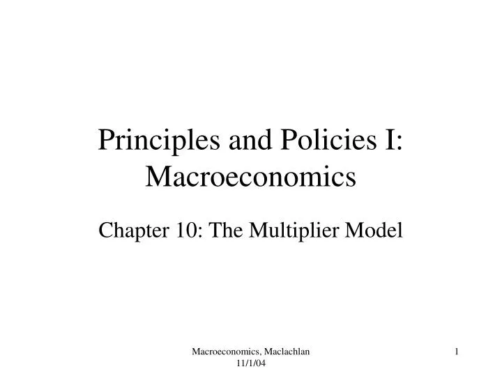
Principles and Policies I: Macroeconomics Chapter 10: The Multiplier Model Macroeconomics, Maclachlan 11/1/04
Chapter 10 Learning ObjectivesYou should be able to … • Explain the difference between induced and autonomous expenditures. • Show how the level of income is graphically determined in the multiplier model. • Use the multiplier equation to determine equilibrium income. • Explain how the multiplier process amplifies shifts in autonomous expenditures. • Demonstrate how fiscal policy can eliminate recessionary and inflationary gaps. • List six reasons why the multiplier model might be misleading. Macroeconomics, Maclachlan 11/1/04
Price level Induced shift (Multiplier effects) Initial shift 20 P0 Aggregate supply ? AD AD Cumulative shift Real output The AS/AD Model When Prices Are Fixed Macroeconomics, Maclachlan 11/1/04
The Circular Flow Macroeconomics, Maclachlan 11/1/04
Aggregate production (production = income) Real production B C A $4,000 Potential income 45º 0 $4,000 Real income The Aggregate Production Curve Macroeconomics, Maclachlan 11/1/04
Aggregate Production curve meets … Aggregate Expenditure = C + I + G + (X-M) Multipler Model Macroeconomics, Maclachlan 11/1/04
Building Aggregate Expenditure Function: Autonomous and Induced Expenditures • Autonomous expenditures – expenditures that do not systematically vary with income. • Induced expenditures – expenditures that change as income changes. Macroeconomics, Maclachlan 11/1/04
Building Aggregate Expenditure Function: The Marginal Propensity to Expend • Marginal propensity to expend (mpe) – the ratio of the change in aggregate expenditures to a change in income. • It is composed of the various relationships between the component of aggregate expenditures. • Its value is greater than 0 and less than 1. • It is the slope of the aggregate expenditure curve. Macroeconomics, Maclachlan 11/1/04
Expenditures Function • Autonomous expenditures is the sum of the autonomous components of expenditures: AE0 = C0 + I0 + G0 + (X0 – M0) • Induced expenditures is the sum of the induced components of expenditures. Macroeconomics, Maclachlan 11/1/04
Real expenditures (AE) (in dollars) Real income (in dollars) Solving for Equilibrium Graphically Aggregate production 14,000 12,000 Aggregate expenditures 10,000 AE = 5,000 + 0.5Y Equilibrium 7,000 5,000 AE0 = 5,000 4,000 10,000 14,000 Macroeconomics, Maclachlan 11/1/04
The Multiplier Equation • Expendituresmultiplier – a number that reveals how much income will change in response to a change in autonomous expenditures. Macroeconomics, Maclachlan 11/1/04
The Circular Flow Model and the Multiplier Process • Not all of the flow of income is spent on domestic goods (the mpe < 1). • This represents a leakage from the circular flow. • Autonomous expenditures are injections into the circular flow. • They offset the leakages. Macroeconomics, Maclachlan 11/1/04
The First Five Steps mpe = .4 mpe = .5 100 100 50 40 25 16 6.4 6.25 12.5 2.56 Multiplier = 1/(1-0.4) = 1.7 Multiplier = 1/(1-0.5) = 2 Macroeconomics, Maclachlan 11/1/04
Real expenditures Aggregate production AE1 $4,210 30 AE0 4,090 1,052.5 30 1,022.5 $120 0 $4,090 $4,210 Real income An Upward Shift of AE Macroeconomics, Maclachlan 11/1/04
Aggregate production AE0 $4,152 AE1 30 4,062 30 1,412 1,382 $90 $4,062 $4,152 An Downward Shift of AE Real expenditures 0 Real income Macroeconomics, Maclachlan 11/1/04
Aggregate production Potential output LAS AE1 AE0 E2 $60 $120 ∆G = $60 mpe = 0.67 SAS AE1 = 333 + 0.67Y E1 AD0 AD1 Recessionary gap AD1΄ $180 $1,000 $1,180 Real income $1,000 $1,180 Real income Fighting Recession: Expansionary Fiscal Policy Initial expenditures increase Multiplier effect McGraw-Hill/Irwin © 2004 The McGraw-Hill Companies, Inc., All Rights Reserved.
Aggregate production Potential output LAS AE0 AE1 P1 B E1 ∆G = $200 $1,000 A mpe = 0.8 SAS P0 AE1 = 800 + 0.8Y AD0 E2 Inflationary gap AD1 $4,000 $5,000 Real income $4,000 $5,000 Real income Fighting Inflation: Contractionary Fiscal Policy McGraw-Hill/Irwin © 2004 The McGraw-Hill Companies, Inc., All Rights Reserved.
Limitations of Multiplier Model • It’s incomplete: needs info on where economy starts and potential output. • It over emphasizes shifts in AE. • It assumes a fixed price level. • It doesn’t consider expectations. • It ignores possibility of desired shifts in AE. • It ignores permanent income hypothesis. Macroeconomics, Maclachlan 11/1/04
Problem 10-1 The mpe is 0.8. Autonomous expenditures are $4,200. What is the equilibrium income in the economy? $21,000 Macroeconomics, Maclachlan 11/1/04
mpe = .6 Multiplier = 2.5 A = 1,000 + 8,000 + 10, 000 + 1,000 = 20,000 Y = 50,000 Increase in A of 2,000 Y increases by 5,000 (or 10%) Unemployment decreases by 5 percentage points. mpe = .5 Multiplier = 2 Y= 40,000 Y increases by 4,000 (or 10%) Unemployment decreases by 5 percentage points. Problem 10-4 Macroeconomics, Maclachlan 11/1/04