Download
1 / 20
200 likes | 455 Views
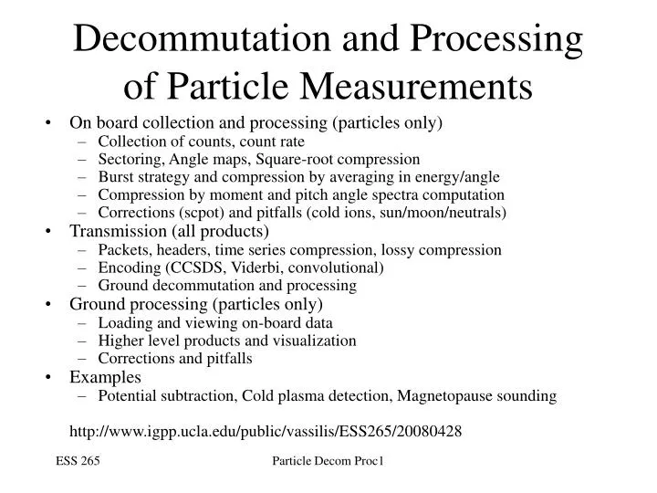
Decommutation and Processing of Particle Measurements. On board collection and processing (particles only) Collection of counts, count rate Sectoring, Angle maps, Square-root compression Burst strategy and compression by averaging in energy/angle

E N D
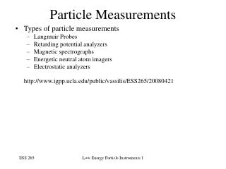
Decommutation and Processing of Particle Measurements • On board collection and processing (particles only) • Collection of counts, count rate • Sectoring, Angle maps, Square-root compression • Burst strategy and compression by averaging in energy/angle • Compression by moment and pitch angle spectra computation • Corrections (scpot) and pitfalls (cold ions, sun/moon/neutrals) • Transmission (all products) • Packets, headers, time series compression, lossy compression • Encoding (CCSDS, Viderbi, convolutional) • Ground decommutation and processing • Ground processing (particles only) • Loading and viewing on-board data • Higher level products and visualization • Corrections and pitfalls • Examples • Potential subtraction, Cold plasma detection, Magnetopause sounding http://www.igpp.ucla.edu/public/vassilis/ESS265/20080428 Particle Decom Proc1
Further reading(in class web site unless otherwise specified) • Curtis et al., On board analysis techniques for space plasma particle instruments, Rev. Sci. Instrum., 60, 372, 1989. • Abiad, R., The ESA and SST (ETC) board requirements specification, 2005. thm_sys_105a_etc_req.1.7.pdf • Carlson, C. W., The square-root compression algorithm, 1993. FAST_ESA_SQRT_compression.doc • Fast-Floating Point: • Description: thm_fsw_221_Floating_Point.doc (by Harvey, P. R.) • Converter: thm_fsw_221_ffp.xls (by Harvey, P. R.) • Huffman, Differencing in: • thm_fsw_900_Compression_Options.doc; thm_fsw_901A_Compression_Huffman.doc • THEMIS analysis software • User’s Guide: ftp://apollo.ssl.berkeley.edu/pub/THEMIS/3%20Ground%20Systems/3.2%20Science%20Operations/Science%20Operations%20Documents/Software%20Users%20Guides/THEMIS_Science_Data_Analysis_Software_Users_Guide.pdf • GEM’07 Tutorial: ftp://apollo.ssl.berkeley.edu/pub/THEMIS/3%20Ground%20Systems/3.2%20Science%20Operations/Science%20Operations%20Documents/Science%20Software%20Data%20Analysis%20Software%20Presentation%20-%20GEM%20Dec%202007/Themis_Science_Software_Demo_Software_GEM_Dec_2007_Rev%20A.ppt Particle Decom Proc2
On board collection/processing • Collection of counts, count rates • Sectoring, Angle maps, Square-root compression • See modes, energy, sector maps in: • class_materials/energy_angle_maps/etcmap_*.xls • Burst strategy and compression by averaging in energy/angle • Compression by moment and pitch angle spectra computation • See: Curtis et al. Rev. Sci. Instr. And • Abiad, technical memo: thm_sys_105a_etc_req1.7.pdf • Corrections (scpot) and pitfalls (cold ions, sun/moon/neutrals) Particle Decom Proc3
Transmission • Packets, headers, time series compression, lossy compression • Encoding (CCSDS, Viterbi, convolutional) • On-board data: Ground decommutation and processing • Moments • L0 (.pkt) and L1 (.cdf) contain same (raw) data in DSL coordinates • L2 (.cdf) contain calibrated data in other coordinates (GSE, GSM) • Particle distributions • L0 packet files • Raw, sqrt-compressed counts (efficient for loading) • Files organized by APID, but transparent to user • L1 CDF files • Raw, uncompressed counts • All quantities in one file • L2 CDF files • Omni-directional spectra (will eventually contain DF’s) • Derived, ground-processed moments in useful coordinates Particle Decom Proc4
Ground processing (particles only) • Loading and viewing on-board processed data • There is a single routine for loading on-board moments • thm_load_mom, level=1 (loads L1 or L2 data) • Products introduced (in either case) • 1 thb_p[e,s,t][i,e]m_density x 6 • 2 thb_peim_flux (particle flux in #/cm2/s) • 3 thb_peim_mftens (momentum flux in eV/ cm3) • 4 thb_peim_eflux (particle flux in #/cm2/s) • 5 thb_peim_velocity (km/s) • 6 thb_peim_ptens (eV/cm3) • 7 thb_peim_ptot (trace of pressure tensor) • … • 43 thb_pxxm_pot (probe potential subtracted, in Volts) • 44 thb_pxxm_qf • 45 thb_pxxm_shft • Note: [e,s,t] correspond to ESA, SST, Total; [i,e] to ions, electrons • E.g., thb_ptim_velocity is the total velocity from the ESA and SST combined • There are two routines for introducing ESA distributions • thm_load_esa_pkt (loads L0 data) • thm_load_esa, level=… (loads L1 and L2 data, will become prime in future) • There is a single routine for introducing SST distributions • thm_load_sst (loads SST L1 data) Particle Decom Proc5
Ground processing (particles only) • Loading and viewing on-board processed data • There is a single routine for loading on-board moments • thm_load_mom, level=1 (loads L1 or L2 data) • There are two routines for introducing ESA distributions • thm_load_esa_pkt (loads all L0 data, introduces spectra) • Products introduced (12 total): omnidirectional spectra • 46 thb_pe[i,e][r,f,b]_en_counts x 6 (spectra) • 47 thb_pe [i,e][r,f,b]_mode x 6 (energy/angle modes) • Note: [i,e] is ions, electrons; [r,f,b] is reduced, full, burst mode • thm_load_esa, level=… (now loads L2 spectra, in the future L1 data as well) • There is a single routine for introducing SST distributions • thm_load_sst (loads SST L1 data) • Generic routines • To “get” any distribution function type: • dat=thm_part_dist(‘thb_peif’,gettime(/c)) • ;or: ctime,t & dat=thm_part_dist(‘thb_peif’,t) • ;or: ctime,t & dat=get_tha_peif(t) • wset,1 & spec3d,dat • wset,2 & plot3d,dat,units=‘counts’ ; convert units • ; other types: eflux,flux,df,rate • To obtain moments type (e.g. n, v, t): • thm_part_spec_calc,probe='b',moments=['density','flux'],instrument=['peif','psif'] • Unit Conversions: • To copy/convert to/from units (eflux,flux,df,counts,rate), use function conv_units: • dat_new=conv_units(dat,‘df’) Particle Decom Proc6
Ground processing (particles only) • Loading and viewing on-board processed data • There is a single routine for loading on-board moments: thm_load_mom, level=1 • There is a main routine for introducing ESA distributions: thm_load_esa_pkt • There is a single routine for introducing SST distributions: thm_load_sst • Generic routines • To “view” distribution function contents type: • dat=thm_part_dist(‘thb_peif’,gettime(/c)) • help, dat, /str • print, dat.energy, dat.theta, dat.phi ; to view energy/angle bin centers ** Structure <13c28790>, 35 tags, length=140952, ….: PROJECT_NAME STRING 'THEMIS' SPACECRAFT STRING 'b' DATA_NAME STRING 'IESA 3D Full' APID INT 454 UNITS_NAME STRING 'counts' UNITS_PROCEDURE STRING 'thm_convert_esa_units' VALID BYTE 1 TIME DOUBLE 1.1746494e+009 ; seconds since 1970 DELTA_T DOUBLE 3.0899630 INTEG_T DOUBLE 0.0030175420 DT_ARR FLOAT Array[32, 88] CONFIG1 BYTE 2 CONFIG2 BYTE 1 AN_IND INT 1 EN_IND INT 1 MODE INT 2 NENERGY INT 32 ENERGY FLOAT Array[32, 88] DENERGY FLOAT Array[32, 88] EFF DOUBLE Array[32, 88] BINS INT Array[32, 88] NBINS INT 88 THETA FLOAT Array[32, 88] DTHETA FLOAT Array[32, 88] PHI FLOAT Array[32, 88] DPHI FLOAT Array[32, 88] DOMEGA FLOAT Array[32, 88] GF FLOAT Array[32, 88] GEOM_FACTOR FLOAT 0.00153000 DEAD FLOAT 1.70000e-007 MASS FLOAT 0.0104389 CHARGE FLOAT 1.00000 SC_POT FLOAT 0.000000 MAGF FLOAT Array[3] DATA FLOAT Array[32, 88] Particle Decom Proc7
Ground processing (particles only) • Loading and viewing on-board processed data • …. • Generic routines • To introduce s/c potential and magnetic field type: • ctime,t & dat=thm_part_dist(‘thb_peif’,t) • get_data,’thb_pxxm_pot’,data=thb_pxxm_pot_str • it=where((thb_pxxm_pot_str.x gt t(0)-3.) and (thb_pxxm_pot_str.x lt t(0)+3.)) • dat.sc_pot=median(thb_pxxm_pot_str.y(it)) • get_data,’thb_fgs_dsl’,data=thb_fgs_dsl_str • jt=where((thb_fgs_dsl_str.x gt t(0)-1.5) and (thb_fgs_dsl_str.x lt t(0)+1.5)) • dat.magf(*)=thb_fgs_dsl_str.y(jt,*) • If sc_pot not available, use a guess (e.g., sc_pot=15V) • dat.sc_pot=-10. ; Volts • Compute the density, temperature for that instant • print,'ion density 1/cc = ',n_3d(dat) • print,'ion temperature eV = ',t_3d(dat) • Another way is to use generic tool to introduce scpot and mag: • thm_part_spec_calc,probe='b',scpot_suffix=‘_pxxm_pot’,mag_suffix=‘_fgs_dsl’, • moments=['density',‘velocity‘,’t3’,’magt3’],instrument=['peif','psif'] Particle Decom Proc8
Ground processing (particles only) • Loading and viewing on-board processed data • Viewing Cuts • Use (crib themis_cut_crib provided in class material: idl/dfcuts): slice2d_themis_longer_esa,sc,typ,current_time,timeinterval,thebdata='th'+sc+'_fgs_dsl',species=species,range=range,rotation=rotation,angle=angle,filetype=filetype,outputfile=outputfile;,nosmooth=1 • Note, rotations: • ; 'BV': x = V_para and the bulk velocity in the x-y plane. (DEFAULT) • ; 'BE': x = V_para and the VxB in the x-y plane. • ; 'xy': x = V_x and y = V_y. • ; 'xz': x = V_x and y = V_z. • ; 'yz': x = V_y and y = V_z. • ; 'perp': x-y plane is perp. to B, x is velocity projection on plane. • ; 'perp_xy': x-y plane is perp. to B, x is x-axis projection on plane. • ; 'perp_xz': x-z plane is perp. to B, y is z-axis projection on plane. • ; 'perp_yz': x-y plane is perp. to B, x is y-axis projection on plane. • Other options (PA vs E) Particle Decom Proc9
Ground processing (particles only) • Higher level products and visualization • Particle spectrograms in various coordinates • DSL coordinates • Energy, theta/phi angle spectrograms • ;DSL coordinates • ; energy spectrogram • thm_part_getspec, probe=['b'], trange=['07-03-23/11:10','07-03-23/11:30'], $ • data_type=['psif'],/energy, $ • phi=[-135,-45], theta=[-45,45], erange=[25000,500000],suff='_dusk' • thm_part_getspec, probe=['b'], trange=['07-03-23/11:10','07-03-23/11:30'], $ • data_type=['psif'],/energy, $ • phi=[45,135], theta=[-45,45], erange=[25000,500000],suff='_dawn' • ; phi spectrogram • thm_part_getspec, probe=['b'], trange=['07-03-23/11:10','07-03-23/11:30'], $ • data_type=['peir'],angle='phi', $ • phi=[0,360], theta=[-90,90], erange=[1.5e4,2.5e4] • ; theta spectrogram • thm_part_getspec, probe=['b'], trange=['07-03-23/11:10','07-03-23/11:30'], $ • data_type=['peir'],angle='theta', $ • phi=[0,360], theta=[-90,90], erange=[1.5e4,2.5e4] • tplot,'thb_fgs_gsm thb_psif_en_eflux_dusk thb_peir_an_eflux_*' • tlimit,['07-03-23/11:12','07-03-23/11:22'] Particle Decom Proc10
Ground processing (particles only) • DSL coordinates • Energy, theta/phi angle spectrograms • ;DSL coordinates (results) Particle Decom Proc11
Ground processing (particles only) • Higher level products and visualization • Particle spectrograms in various coordinates • FAC coordinates (field aligned) • Energy, pitch angle (pa) / gyro(velocity)phase angle spectrograms • ; Energy spectrogram • thm_part_getspec, probe=['b'], trange=['07-03-23/11:10','07-03-23/11:30'],$ • data_type=['psif'], /energy, $ • pitch=[0,45], suff='_para', $ • erange=[25000,500000],regrid=[32,16] • ; Gyro(velocity)phase spectrogram • thm_part_getspec, probe=['b'], trange=['07-03-23/11:10','07-03-23/11:30'],$ • data_type=['psif'], angle='gyro', $ • pitch=[45,135], other_dim='ygsm', suff='_perp', $ • erange=[100000,150000],regrid=[32,16] • ; Pitch angle spectrogram • thm_part_getspec, probe=['b'], trange=['07-03-23/11:10','07-03-23/11:30'],$ • data_type=['peer'], angle='pa', $ • erange=[15000,25000],regrid=[32,16] • tplot,'thb_fgs_gsm thb_psif_en_eflux_para thb_psif_an_eflux_gyro_perp thb_peer_an_eflux_pa' • tlimit,['07-03-23/11:12','07-03-23/11:22'] Particle Decom Proc12
Ground processing (particles only) • FAC coordinates (field aligned) • Energy, pitch angle (pa) / gyro(velocity)phase angle spectrograms (results) Particle Decom Proc13
Ground processing (particles only) • Higher level products and visualization • Particle spectrograms in various coordinates • FAC coordinates (field aligned) (Look in: thm_fac_matrix_make) • other_dimension: • ; 'Xgse', (DEFAULT) translates from gse or gsm into FAC • ; Definition(works on GSE, or GSM): X Axis = on plane defined by Xgse - Z • ; Second coordinate definition: Y = Z x X_gse • ; Third coordinate, X completes orthogonal RHS • ; 'Rgeo',translate from geo into FAC using radial position vector • ; Rgeo is radial position vector, positive radialy outwards. • ; Second coordinate definition: Y = Z x Rgeo (westward) • ; Third coordinate, X completes orthogonal RHS XYZ. • ; 'mRgeo', opposite to above • ; mRgeo is radial position vector, positive radially inwards. • ; 'Phigeo', translate into FAC using azimuthal position vector • ; Phigeo is the azimuthal geo position vector, positive Eastward • ; First coordinate definition: X = Phigeo x Z (positive outwards) • ; Second coordinate, Y ~ Phigeo (eastward) completes orthogonal RHS XYZ • ; 'mPhigeo', opposite to above • ; Second coordinate, Y ~ mPhigeo (Westward) completes orthogonal RHS XYZ • ; 'Phism', translate into FAC using azimuthal Solar Magnetospheric vector. • ; Phism is "phi" vector of satellite position in SM coordinates. • ; Y Axis = on plane defined by Phism-Z, normal to Z • ; Second coordinate definition: X = Phism x Z; Third completes orthogonal RHS; ; 'mPhism', opposite to above • ; mPhism is minus "phi" vector of satellite position in SM coordinates. • ; 'Ygsm', translate into FAC using cartesian Ygsm position as other dimension. • ; Y Axis on plane defined by Ygsm and Z • ; First coordinate definition: X = Ygsm x Z • ; Third completes orthogonal RHS XYZ Particle Decom Proc14
Ground processing (particles only) • Pitfalls • Sun contamination • ; Sun contamination • ; • trange=['08-02-22/04:40','08-02-22/05:00'] • timespan,'08-02-22/04:00',1,/hours • sc='c‘ • thm_load_fgm,probe=sc,data='fgl',coord='dsl gsm' • thm_part_getspec, probe=sc,trange=trange, $ • theta=[0,45], phi=[0,360], start_angle=-180., $ • erange=[25000,40000], data_type=['psif'], $ • suffix='_ne',angle=phi • thm_part_getspec, probe=sc,trange=trange, $ • theta=[-45,0], phi=[0,360], start_angle=-180., $ • erange=[25000,40000], data_type=['psif'], $ • suffix='_se',angle=phi • tplot,'thc_fgl_dsl thc_fgl_gsm thc_psif_an_eflux_phi_ne thc_psif_an_eflux_phi_se' • tlimit,['08-02-22/04:40','08-02-22/05:00'] Particle Decom Proc15
Ground processing (particles only) • Pitfalls • Sun contamination • ; Sun contamination Particle Decom Proc16
Ground processing (particles only) • Pitfalls • Sun contamination: Bin removal • ; • edit3dbins,thm_sst_psif(probe=sc, gettime(/c)), bins2mask • ; ON: Button1; OFF: Button2; QUIT: Button3 • bins2mask = where(bins2mask eq 0) • print,bins2mask • thm_part_getspec, probe=sc,trange=trange, $ • theta=[0,45], phi=[0,360], start_angle=-180., $ • erange=[25000,40000], data_type=['psif'], $ • suffix='_ne',angle=phi,bins2mask=bins2mask • ; • thm_part_getspec, probe=sc,trange=trange, $ • theta=[-45,0], phi=[0,360], start_angle=-180., $ • erange=[25000,40000], data_type=['psif'], $ • suffix='_se',angle=phi,bins2mask=bins2mask • ; • tplot Particle Decom Proc17
Ground processing (particles only) • Pitfalls • Sun contamination: Bin removal • ; Particle Decom Proc18
Homework • Find a THEMIS interval of interest to your research • Plot one energy, phi, theta spectrogram from ESA and SST • Plot one pitch, gyrophase spectrogram from ESA and SST • Plot ESA ion and electron distribution functions in • Vpar, perp and in XY coordinates • Cold plasma detection Particle Decom Proc19
Topics for May 14/May 19 class • Potential subtraction • Cold plasma detection • Magnetopause sounding Particle Decom Proc20