Download
1 / 14
180 likes | 614 Views
Chapter 7 – The Choropleth Map. Data Classification. Appropriateness of Data. Enumeration mapping – describes areal classified or aggregated data Appropriateness of Data – political boundary (Census Bureau units) Not appropriate – continuous phenomena should not be mapped by choropleth maps

E N D
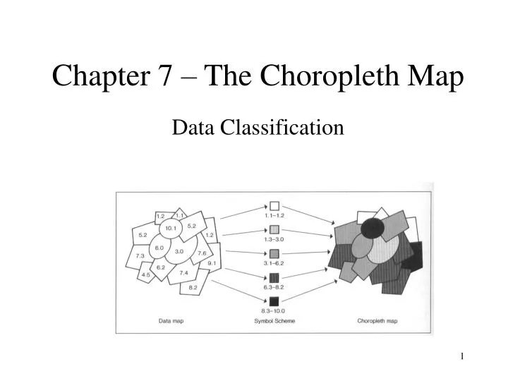
Chapter 7 – The Choropleth Map Data Classification
Appropriateness of Data • Enumeration mapping – describes areal classified or aggregated data • Appropriateness of Data – political boundary (Census Bureau units) • Not appropriate – continuous phenomena should not be mapped by choropleth maps • Two enumeration data: totals or derived. • Sometimes, totals are not suitable for mapping (Fig 7.4) • Major Assumption – the value in the enumeration unit is spread uniformly throughout the unit. • If data cannot be dealt with as ratios or proportions, then should not be portrayed by the choropleth tecnique.
Common Methods of Data Classification • No more than 5 to 7 classes • Six common methods - equal intervals, standard deviation, Arithmetic progression, Geometric progression, Quantile, Natural breaks, and optimal.
Equal Intervals • Useful when histogram of data array has a rectangular shape (rare in geographic phenomena) • Advantages: 1) easy to compute the intervals 2) easy to interpret the resulting intervals 3) no gap in the legend display 4) only lowest limits can be shown in legend • Disadvantage: skewed data is not appropriate.
Calculating Steps • 1. Calculate the range of the data (R) : R = H – L • 2. Obtain the common difference (CD) : CD = R/(# of Classes) • 3. Obtain the class limits by calculating • L + 1 x CD = first class limit • L + 2 x CD = second class limit • L + (n-1) x CD = last class limit
Quantile • Ordered data are placed in classes. • Ties can complicate the quantiles method. • Advantages - 1) class limits can be computed manually.2) if enumeration units are same, each class will have the same map area. 3) quantile are useful for ordinal-level data, no numeric information would be necessary to create the classification. • Disadvantage - 1) gap result may vary. 2) fails to consider data distribution. • K = # of enumeration units / number of classes
Standard Deviation • Used only when the data array approximates a normal distribution. • Advantages: 1) Distribution of data is taken into account. 2) if normal distributed data is used, the mean is a good divider. 3) no gap in the legend. • Disadvantage: 1) only work with normal-distributed data. 2) negative values may be in the range
Geometric Progression • Useful technique when frequency of data declines continuously with increasing magnitude • a, ar1, ar2, ...arn • 1) compute common multiplier (a is the lowest value, r is the common multiplier and n is the number of classes • use “Xmin x rn = Xmax” to obtain r • eg. 118 x r5 = 790 ( use Area as variable) r = 1.46 • So the interval goes from • 118, 118x1.46, 118x1.462, 118x1.463,118x1.464 • 118-172, 173-252, 253-367, 368-536, 537-790
Graphic Array • Figure 7.11 • Class boundaries are identified at places where slopes change remarkably • Disadvantage: not suitable for large amount of data
Jenks Optimization • Forming groups that are internally homogenous while assuring heterogeneity among classes • groups are created based on gaps. • Minimize differences within class and maximize differences between classes. • Based on GVF (Goodness of Variance Fit) - an optimization techniques to minimize the sum of the variance within each of the class.
GVF (Fisher-Jenkins Algorithms) • 1) compute the squared deviation of each data • Compute SDCM (Squared Deviation, Class Means). • Compute GVF = (SDAM - SDCM) / SDAM • The goal is to maximize the value of GVF (closer to 1.0 is the better value)
Practice • Copy US-states2.xls from g:\4210\data\ to your own folder. (you may need to create a folder under hw and have this file copied to) • Compute 5 classes intervals of “Pop90_sqmi” for the following methods • Geometric Progression • Quantile • Equal Interval • GVF (use GIS’s range to compute GVF)
Practice - ArcMap • Open a new project and add states.shp from c:\esri\esridata\usa to the layer • Plot the US map based on Pop90_sqmi using different methods. • Compute GVFs for the four methods.