Download
1 / 29
430 likes | 2.57k Views
Structural Geology (3443) Lab 2 – Contour Maps . Department of Geology University of Texas at Arlington. Any scalar value that changes with position can be contoured. Elevation of the Earth Thickness of sediment Chemical species in groundwater Depth to a geological formation Etc.

E N D
Structural Geology (3443)Lab 2 – Contour Maps Department of Geology University of Texas at Arlington
Any scalar value that changes with position can be contoured. Elevation of the Earth Thickness of sediment Chemical species in groundwater Depth to a geological formation Etc. Lab 2 – Contour Maps
Earth’s topography is typical. A contour line represents contiguous points that are of equal distance above a reference plane. Mean sea level is the usual reference. The contour interval is constant and is distance between adjacent contours. What is the contour interval of the fig? Index Contours. Lab 2 – Contour Maps
Lab 2 – Contour Maps Reading Contour Maps Identify data peaks, ridges, valleys, saddles, depressions.
Data Gradient (slope fraction) is defined as dz/dl, or as rise/run in Fig. 2-4, which is a vertical cross-section through the data. The slope angle, f, is arctan(gradient) The grade is just the % gradient. What is the grade or a 45o slope? A 90o slope? Lab 2 – Contour Maps
Lab 2 – Contour Maps If the contour interval is constant, what is the relationship between data gradient (slope angle) and contour spacing
Lab 2 – Contour Maps Where are the flatter areas and the steeper areas on the topo map? What are the black squares?
Lab 2 – Contour Maps Constraints Contour interval is constant Contour lines do not merge or cross (overhangs excepted) Contour lines form closed loops unless they hit a discontinuity (like the edge of the map) A Datum plane must be specified (e.g. mean sea level)
Interpreting topographic maps The Earth’s land surface is produced by weathering and erosion of rocks. Rocks and structural features have different weathering and erosion characteristics, so the topography reflects the underlying geology. Elevated areas are resistant to erosion, low areas less resistant. Lab 2 – Contour Maps
Lab 2 – Contour Maps This area of the Appalachians in Pennsylvania is a classic example of topography showing the geology.
Intersection of planes (strata) with topography: Rule of V’s Lab 2 – Contour Maps
Intersection of planes (strata) with topography: Rule of V’s Lab 2 – Contour Maps
Lab 2 – Contour Maps Intersection of planes (strata) with topography: Rule of V’s
If the strata is folded (curved) and not planar, then intersection of the strata with topography is much more complicated Lab 2 – Contour Maps
Instead of topography, we can contour the top of a formation. This is called a structure contour map because it shows the ups and downs of the formation in the subsurface. The next slide shows a structure contour maps of the Permian Wolfcamp formation. Lab 2 – Contour Maps
Lab 2 – Contour Maps The datum is sea level; the blues are deepest and reds & violet are shallow.
Faults (discontinuities) are represented on structure contour maps as breaks in the contours. Lab 2 – Contour Maps
Lab 2 – Contour Maps Faults are difficult to detect based on contours alone. Is it a fault, or just steeply dipping layers?
Other examples of structure contours Lab 2 – Contour Maps
In addition to structure maps, we can also contour the thickness of a sedimentary formation. These are called Isopach maps Remember, thickness is the perpendicular distance between the layer boundaries, so if the layer is tilted, the thickness is not the same as the vertical distance. Lab 2 – Contour Maps
Thickness in the subsurface is often obtained from vertical wells. Uncorrected thicknesses from wells used in contour maps are called isochore maps These are not reliable thickness maps. Lab 2 – Contour Maps
Faults can also affect thickness measurements. Reverse faults thicken horizontal layers Normal faults thin horizontal layers. Lab 2 – Contour Maps
Constructing contour maps Topographic maps are usually constructed from stereo pairs of aerial photos which provide a 3-D image of the ground. These map are quite accurate because there are almost an infinite number of data points. 3-D seismic images, like stereo aerial photos, can also provide accurate structural contour maps in 2-way travel time. (Seismic methods measure travel time, not depth). The time can be converted to depth knowing the acoustic velocity of the rock, but that is not known very well, so depths from seismic data are usually inaccurate. Lab 2 – Contour Maps
Lab 2 – Contour Maps Constructing contour maps Usually, data for stratigraphic thickness and depth to a formation top comes from well information. Because well information is sparse and not uniformly distributed, this point data must be interpolated and extrapolated, so these contour maps are less reliable. Three methods are commonly used to construct contours: Objective: Strict interpolation used Parallel: contours are kept parallel, strict interpolation is violated Interpretative: only the interpreter’s judgment is used – his/her “feeling” of what the surface should like. Interpolation between points is qualitative.
Lab 2 – Contour Maps In all methods of contouring, the rules of contours must be followed: Contour interval is constant Different contour lines do not merge or cross (overhangs excepted). A contour line may join itself to form a closed loop Contour lines always form closed loops unless they hit a discontinuity (like the edge of the map or a fault) A Datum plane must be specified (e.g. mean sea level)
We will use both the objective method, which most computer contouring programs use, and the interpretative method. A contour interval is selected that does not give more resolution than the number of data points provides. Interpolation lines are drawn between each point and its nearest neighbor. The elevation of each contour is drawn on each line assuming the slope is constant along the line. Lab 2 – Contour Maps
We will use a cm ruler and calculator to interpolate. Imagine vertical triangle between points 40 & 199. Measure map distance between the points Elevation change along baseline – 3.975/mm Find location of 60 contour: = (60-40)/3.975 = 5.03mm from point 40 Location of 180 contour = (180-40)/3.975 = 35.22 mm Lab 2 – Contour Maps
Lab 2 – Contour Maps When all the contours have been interpolated, then the contours can be drawn in. Where does the 80 contour go?
Example contours from data. Lab 2 – Contour Maps