Download
1 / 14
140 likes | 1.1k Views
Ch 6.4: Differential Equations with Discontinuous Forcing Functions . In this section, we focus on examples of nonhomogeneous initial value problems in which the forcing function is discontinuous. Example 1: Initial Value Problem (1 of 12). Find the solution to the initial value problem

E N D
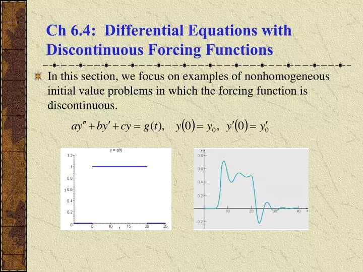
Ch 6.4: Differential Equations with Discontinuous Forcing Functions • In this section, we focus on examples of nonhomogeneous initial value problems in which the forcing function is discontinuous.
Example 1: Initial Value Problem (1 of 12) • Find the solution to the initial value problem • Such an initial value problem might model the response of a damped oscillator subject to g(t), or current in a circuit for a unit voltage pulse.
Example 1: Laplace Transform (2 of 12) • Assume the conditions of Corollary 6.2.2 are met. Then or • Letting Y(s) = L{y}, • Substituting in the initial conditions, we obtain • Thus
Example 1: Factoring Y(s) (3 of 12) • We have where • If we let h(t) = L-1{H(s)}, then by Theorem 6.3.1.
Example 1: Partial Fractions (4 of 12) • Thus we examine H(s), as follows. • This partial fraction expansion yields the equations • Thus
Example 1: Completing the Square (5 of 12) • Completing the square,
Example 1: Solution (6 of 12) • Thus and hence • For h(t) as given above, and recalling our previous results, the solution to the initial value problem is then
Example 1: Solution Graph (7 of 12) • Thus the solution to the initial value problem is • The graph of this solution is given below.
Example 2: Initial Value Problem (1 of 12) • Find the solution to the initial value problem • The graph of forcing function g(t) is given on right, and is known as ramp loading.
Example 2: Laplace Transform (2 of 12) • Assume that this ODE has a solution y = (t) and that '(t) and ''(t) satisfy the conditions of Corollary 6.2.2. Then or • Letting Y(s) = L{y}, and substituting in initial conditions, • Thus
Example 2: Factoring Y(s) (3 of 12) • We have where • If we let h(t) = L-1{H(s)}, then by Theorem 6.3.1.
Example 2: Partial Fractions (4 of 12) • Thus we examine H(s), as follows. • This partial fraction expansion yields the equations • Thus
Example 2: Solution (5 of 12) • Thus and hence • For h(t) as given above, and recalling our previous results, the solution to the initial value problem is then
Example 2: Graph of Solution (6 of 12) • Thus the solution to the initial value problem is • The graph of this solution is given below.