Techniques for Time Series Analysis_ ARIMA, Exponential Smoothing, Seasonal Decomposition

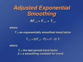
1. Techniques for Time Series Analysis: ARIMA, Exponential Smoothing, SeasonalDecomposition • 1.ARIMA(AutoregressiveIntegratedMovingAverage): • ComponentsofARIMA: • Autoregressive(AR):Uses pastvalues tomodel thecurrent valueof theseries. • Integrated (I): Involvesdifferencing the datato makeit stationary. • Moving Average (MA):Uses pastforecast errors tomodel thecurrent value. • ModelSelection: • UsetheACF(AutocorrelationFunction)andPACF(PartialAutocorrelationFunction)plots toidentify the appropriate lagsfor AR and MA components.Data Science Course. • ModelFittingandValidation: • FittheARIMAmodelusingsoftwaretoolslike R(auto.arimafunction)orPython (statsmodelslibrary).Validatethemodelbycheckingresidualplotsforrandomnessand performingout-of-sample forecasts. • 2.ExponentialSmoothing: • SimpleExponentialSmoothing: • -Suitablefortimeseriesdatawithouttrendsorseasonality.Itappliesexponentially decreasingweights to past observations. • Holt’sLinearTrend Model: • -Extendssimpleexponentialsmoothingbyaddingacomponenttomodelthe trend.Useful fordata with a linear trend. • Holt-WintersSeasonalModel: • FurtherextendsHolt’smodeltoincludeseasonality.Canbeadditiveormultiplicative, dependingon the nature of the seasonalcomponent. • SmoothingParameters: • Parametersalpha(level),beta(trend),andgamma(seasonality)controlthesmoothing process.These can be optimized using software toolsto best fit the data. • 3.SeasonalDecompositionof TimeSeries(STL): • -ComponentsofDecomposition: • -TrendComponent:Representsthelong-termprogressionofthe series.

2. SeasonalComponent:Capturesrepeatingshort-termcyclesorpatterns.SeasonalComponent:Capturesrepeatingshort-termcyclesorpatterns. • Residual Component: Represents random noise or irregular patterns after removing trend andseasonality. • Additivevs.MultiplicativeDecomposition: • Use additive decomposition when the seasonal variations are roughly constant over time. Use multiplicative decomposition when the seasonal variations change proportionally with the levelof the series. • Implementation: • Tools like R (decompose and stl functions) and Python (statsmodels' seasonal_decompose function)can be used to perform STLdecomposition. • 4.ModelEvaluationandSelection: • PerformanceMetrics: • -UsemetricslikeMeanAbsoluteError(MAE),MeanSquaredError(MSE),andMean AbsolutePercentage Error (MAPE) toevaluate model performance. • Cross-Validation: • - Implement techniques like rolling forecasting origin or time series cross-validation to assess therobustness of your models. • 5.ApplicationsandUseCases: • Forecasting: • -UseARIMAandexponentialsmoothing modelsforshort-term andlong-term forecastingin variousdomains such asfinance, inventory management, andsales forecasting. • AnomalyDetection: • -Decompositiontechniqueshelpinidentifyinganomaliesbyanalyzingtheresidual componentafter removing trend and seasonality. • TrendAnalysis: • -DecompositionandARIMAmodelsaidinunderstandingunderlyingtrendsandseasonal patterns,providing insights for strategicplanning and decision-making. • AdditionalTips: • -StationarityCheck: • - Ensure the time series data is stationary before applying ARIMA models. Use transformations like differencing and logarithms if necessary.

3. -ModelDiagnostics: -Afterfittingamodel,alwayscheckresidual diagnostics toensure there are nopatterns left in theresiduals, indicating a good fit.Data Science Course in Mumbai. These pointers provide a foundational understanding of key techniques in time series analysis, emphasizing practical application and model validation for accurate forecasting and insightful analysis. Businessname:ExcelR-Data Science, Data Analytics, Business Analytics Course Training Mumbai Address:304,3rdFloor,PratibhaBuilding.ThreePetrolpump,LalBahadurShastriRd, oppositeManas Tower, Pakhdi, Thane West, Thane, Maharashtra 400602 Phone:09108238354, Email:enquiry@excelr.com