Download
1 / 61
620 likes | 981 Views
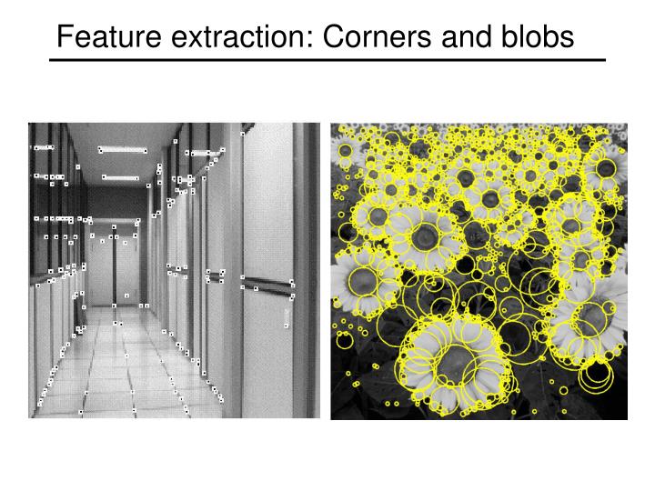
Feature extraction: Corners and blobs. Why extract features?. Motivation: panorama stitching We have two images – how do we combine them?. Step 2: match features. Why extract features?. Motivation: panorama stitching We have two images – how do we combine them?. Step 1: extract features.

E N D
Why extract features? • Motivation: panorama stitching • We have two images – how do we combine them?
Step 2: match features Why extract features? • Motivation: panorama stitching • We have two images – how do we combine them? Step 1: extract features
Why extract features? • Motivation: panorama stitching • We have two images – how do we combine them? Step 1: extract features Step 2: match features Step 3: align images
Characteristics of good features • Repeatability • The same feature can be found in several images despite geometric and photometric transformations • Saliency • Each feature has a distinctive description • Compactness and efficiency • Many fewer features than image pixels • Locality • A feature occupies a relatively small area of the image; robust to clutter and occlusion
Applications • Feature points are used for: • Motion tracking • Image alignment • 3D reconstruction • Object recognition • Indexing and database retrieval • Robot navigation
Finding Corners • Key property: in the region around a corner, image gradient has two or more dominant directions • Corners are repeatable and distinctive C.Harris and M.Stephens. "A Combined Corner and Edge Detector.“Proceedings of the 4th Alvey Vision Conference: pages 147--151.
“flat” region:no change in all directions “edge”:no change along the edge direction “corner”:significant change in all directions The Basic Idea • We should easily recognize the point by looking through a small window • Shifting a window in anydirection should give a large change in intensity Source: A. Efros
Window function Shifted intensity Intensity Window function w(x,y) = or 1 in window, 0 outside Gaussian Harris Detector: Mathematics Change in appearance for the shift [u,v]: Source: R. Szeliski
Harris Detector: Mathematics Change in appearance for the shift [u,v]: Second-order Taylor expansion of E(u,v) about (0,0) (bilinear approximation for small shifts):
M Harris Detector: Mathematics The bilinear approximation simplifies to where M is a 22 matrix computed from image derivatives:
Interpreting the second moment matrix The surface E(u,v) is locally approximated by a quadratic form. Let’s try to understand its shape.
Interpreting the second moment matrix First, consider the axis-aligned case (gradients are either horizontal or vertical) If either λ is close to 0, then this is not a corner, so look for locations where both are large.
direction of the fastest change direction of the slowest change (max)-1/2 (min)-1/2 General Case Since M is symmetric, we have We can visualize M as an ellipse with axis lengths determined by the eigenvalues and orientation determined by R Ellipse equation:
Interpreting the eigenvalues Classification of image points using eigenvalues of M: 2 “Edge” 2 >> 1 “Corner”1 and 2 are large,1 ~ 2;E increases in all directions 1 and 2 are small;E is almost constant in all directions “Edge” 1 >> 2 “Flat” region 1
Corner response function α: constant (0.04 to 0.06) “Edge” R < 0 “Corner”R > 0 |R| small “Edge” R < 0 “Flat” region
Harris detector: Steps • Compute Gaussian derivatives at each pixel • Compute second moment matrix M in a Gaussian window around each pixel • Compute corner response function R • Threshold R • Find local maxima of response function (nonmaximum suppression)
Harris Detector: Steps Compute corner response R
Harris Detector: Steps Find points with large corner response: R>threshold
Harris Detector: Steps Take only the points of local maxima of R
Invariance • We want features to be detected despite geometric or photometric changes in the image: if we have two transformed versions of the same image, features should be detected in corresponding locations
Models of Image Change • Geometric • Rotation • Scale • Affinevalid for: orthographic camera, locally planar object • Photometric • Affine intensity change (I aI + b)
Harris Detector: Invariance Properties • Rotation Ellipse rotates but its shape (i.e. eigenvalues) remains the same Corner response R is invariant to image rotation
Intensity scale:I aI R R threshold x(image coordinate) x(image coordinate) Harris Detector: Invariance Properties • Affine intensity change • Only derivatives are used => invariance to intensity shiftI I+b Partially invariant to affine intensity change
Harris Detector: Invariance Properties • Scaling Corner All points will be classified as edges Not invariant to scaling
Scale-invariant feature detection • Goal: independently detect corresponding regions in scaled versions of the same image • Need scale selection mechanism for finding characteristic region size that is covariant with the image transformation
Recall: Edge detection Edge f Derivativeof Gaussian Edge = maximumof derivative Source: S. Seitz
Edge detection, Take 2 Edge f Second derivativeof Gaussian (Laplacian) Edge = zero crossingof second derivative Source: S. Seitz
maximum From edges to blobs • Edge = ripple • Blob = superposition of two ripples Spatial selection: the magnitude of the Laplacianresponse will achieve a maximum at the center ofthe blob, provided the scale of the Laplacian is“matched” to the scale of the blob
original signal(radius=8) increasing σ Scale selection • We want to find the characteristic scale of the blob by convolving it with Laplacians at several scales and looking for the maximum response • However, Laplacian response decays as scale increases: Why does this happen?
Scale normalization • The response of a derivative of Gaussian filter to a perfect step edge decreases as σ increases
Scale normalization • The response of a derivative of Gaussian filter to a perfect step edge decreases as σ increases • To keep response the same (scale-invariant), must multiply Gaussian derivative by σ • Laplacian is the second Gaussian derivative, so it must be multiplied by σ2
Scale-normalized Laplacian response maximum Effect of scale normalization Original signal Unnormalized Laplacian response
Blob detection in 2D • Laplacian of Gaussian: Circularly symmetric operator for blob detection in 2D
Blob detection in 2D • Laplacian of Gaussian: Circularly symmetric operator for blob detection in 2D Scale-normalized:
Scale selection • At what scale does the Laplacian achieve a maximum response for a binary circle of radius r? r image Laplacian
Scale selection • The 2D Laplacian is given by • Therefore, for a binary circle of radius r, the Laplacian achieves a maximum at (up to scale) Laplacian response r scale (σ) image
Characteristic scale • We define the characteristic scale as the scale that produces peak of Laplacian response characteristic scale T. Lindeberg (1998). "Feature detection with automatic scale selection."International Journal of Computer Vision30 (2): pp 77--116.
Scale-space blob detector • Convolve image with scale-normalized Laplacian at several scales • Find maxima of squared Laplacian response in scale-space
Efficient implementation • Approximating the Laplacian with a difference of Gaussians: (Laplacian) (Difference of Gaussians)
Efficient implementation David G. Lowe. "Distinctive image features from scale-invariant keypoints.”IJCV 60 (2), pp. 91-110, 2004.