Download

1 / 30
300 likes | 376 Views
Equilibrium in Aggregate Economy. Equilibrium in the Aggregate Economy. Changes in the SAS , AD , and LAS curves affect short-run and long-run equilibrium. Short-Run Equilibrium. Short-run equilibrium is where the AS and AD curves intersect. Short-Run Equilibrium.

E N D
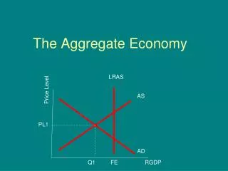
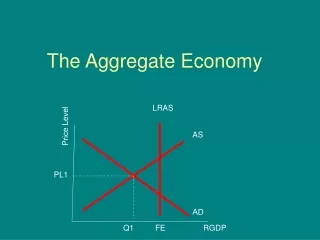
Equilibrium in the Aggregate Economy • Changes in the SAS, AD, and LAS curves affect short-run and long-run equilibrium.
Short-Run Equilibrium • Short-run equilibrium is where the AS and AD curves intersect.
Short-Run Equilibrium • Increases (decreases) in aggregate demand lead to higher (lower) real output and higher (lower) price level. • Upward (downward) shift the SAS curve lead to lower (higher) real output and higher (lower) price level.
P1 F P0 E AD1 AD0 Y1 Y0 Short-Run Equilibrium • Short-run equilibrium is • where SAS = AD0 (point • E). Equilibrium output is • Y0 and the price level is • P0. Price level SAS • If AD increases to AD1, • equilibrium output • increases to Y1 and the • price level increases to P1. P0 E AD0 Y0 Real output
SAS1 G P1 SAS0 E P0 Y0 Y1 Short-Run Equilibrium • Short-run equilibrium is • where SAS0 = AD (point • E). Equilibrium output is • Y0 and the price level is • P0. Price level SAS0 • If SAS increases to SAS1, • equilibrium output • decreases to Y1 and the • price level increases to P1 • (point G). E P0 AD Y0 Real output
Long-Run Equilibrium • Long-run equilibrium is where the AD and long-run aggregate supply curves intersect. • In the long run, output is fixed and the price level is variable.
Long-Run Equilibrium • Aggregate demand determines the price level. • Increases (decreases) in aggregate demand lead to higher (lower) prices.
LAS Price level H P1 E P0 AD1 AD0 Y0 Real output Long-Run Equilibrium:Shift in Aggregate Demand
H P1 AD1 Long-Run Equilibrium LAS Price level • Long-run equilibrium is • point E where AD0 = LAS. • Equilibrium output is at • potential output YP and • the price level is Po. • An increase in AD to AD1 • increases the price level • to P1 but output is un- • changed at YP. E P0 AD0 • In the long-run output is • fixed, and the price level • is variable. YP Real output
Integrating the Short-Run and Long-Run Frameworks • The economy is in both short-run and long-run equilibrium when all three curves intersect in the same location.
Integrating the Short-Run and Long-Run Frameworks • The ideal situation is for aggregate demand to grow at the same rate as aggregate supply and potential output. • Unemployment and growth are at their target rates with no inflation.
Integrating Short-Run and Long-Run Equilibrium • The economy is in long-run and short-run equilibrium at point E where AD=SAS=LAS and output is YP and the price level is P0. LAS SAS E Price level • AD grows at the same rate as potential output, so that unemployment and inflation are very low. P0 AD YP Real output
SAS0 A P0 B SAS1 P1 Y1 Recessionary Gap • Arecessionary gap is the amount by which equilibrium output is below potential output. LAS • If the economy is at point A, some resources are unemployed and the recessionary gap is YP – Y1. SAS0 A P0 • If resources are unemployed for a long time, eventually wages and prices decrease. SAS shifts down to SAS1 and the economy is in long-run and short-run equilibrium at B. Price level AD Recessionary gap Y1 YP Real output
The Recessionary Gap • If the economy remains at this level for a long time, there would be an excess supply of factors of production. • Costs and wages would tend to fall.
SAS2 D P2 C SAS0 P0 Y2 Inflationary Gap • An inflationary gap is the amount by which equilibrium output is above potential output. LAS Price level • If the economy is at point C, resources are being used beyond their potential and the inflationary gap is YP – Y2. C SAS0 P0 AD • If resources are used beyond their potential, eventually wages and prices increase. SAS shifts up to SAS2 and the economy is in long-run and short-run equilibrium at D at a higher price level, P2. Inflationary gap YP Real output Y2
The Inflationary Gap • The inflationarygap occurs when the economy is above potential that exists at the current price level. • Factor prices rise causing the SAS curve to shift up. • The price level rises, and the inflationary gap is eliminated.
The Economy Beyond Potential • When the economy operates below its potential, firms can hire additional factors of production without increasing production costs. • Once the economy reaches its potential output, that is no longer possible.
The Economy Beyond Potential • As firms compete for resources, costs rise beyond productivity increases. • The short-run AS curve shifts up and the price level rises.
The Economy Beyond Potential • The economy will slow down by itself or the government will step in with a policy to contract output and eliminate the inflationary gap.
B P1 AD1 YP Expansionary Fiscal Policy Price level • If the economy is at equilibrium at point A, there is a recessionary gap Y0 – YP. LAS • The appropriate fiscal policy is to increase government spending and/or decrease taxes. SAS P0 A A • AD increases to AD1 and output returns to potential output YP and prices increase slightly to P1. AD0 Y0 Real output
AD2 Contractionary Fiscal Policy LAS • If the economy is at equilibrium at point B, there is an inflationary gap Y2 – YP. • The appropriate fiscal policy is to decrease government spending and/or increase taxes. B AS P2 Price level AD0 • AD decreases to AD2 and output returns to potential output YP and inflation is prevented. YP Y2 Real output
Macro Policy Is More Complicated Than It Looks • Using the AS/AD model to analyze the economy is more complicated than it looks. • Implementing fiscal policy. • Estimating potential output. • Effectiveness of fiscal policy.
The Problem of Implementing Fiscal Policy • There is no guarantee that government will do what the economy needs to be done. • Implementing government spending and tax changes is a slow legislative process. • Government spending and tax decisions are made for political rather than for economic reasons.
The Problem of Estimating Potential Output • Increasing AD when the economy is operating at its potential will accelerate inflation by shifting up the SAS curve.
The Problem of Estimating Potential Output • One way of estimating potential output is to estimate the target rate of unemployment. • Targetrateofunemployment – the rate below which inflation began to accelerate in the past.
The Problem of Estimating Potential Output • Unfortunately, the target rate of unemployment fluctuates and is difficult to predict. • For example, there is structural but no cyclical unemployment at potential output – it is difficult to differentiate between the two.
The Problem of Estimating Potential Output • Another way to determine potential output is to add the normal growth factor (3%) the economy’s previous level. • Estimating the economy’s potential from past growth rates is complicated.
The Questionable Effectiveness of Fiscal Policy • The effectiveness of fiscal policy depends on the government’s ability to perceive a problem and react appropriately to it.
The Questionable Effectiveness of Fiscal Policy • Countercyclical fiscal policy – fiscal policy in which the government offsets any change in aggregate expenditures that would create a business cycle.