Download
1 / 96
960 likes | 964 Views
This study explores an odd categorization asymmetry observed in 3-4 month old infants and explains it using a connectionist auto-encoder model. The model made accurate predictions and highlights how reduced visual acuity in young infants can aid in basic-level categorization.

E N D
Using auto-encoders to model early infant categorization: results, predictions and insights
Overview • An odd categorization asymmetry was observed in 3-4 month old infants. • We explain this asymmetry using a connectionist auto-encoder model. • Our model made a number of predictions, which turned out to be correct. • We used a more neurobiologically plausible encoding for the stimuli. • The model can now show how young infants’ reduced visual acuity may actually help them do basic-level categorization.
Background on infant statistical category-learning Quinn, Eimas, & Rosenkrantz (1993) noticed a rather surprising categorization asymmetry in 3-4 month old infants: • Infants familiarized on cats are surprised by novel dogs • BUT infants familiarized on dogs are bored by novel cats.
How their experiment worked Familiarization phase: infants saw 6 pairs of pictures of animals, say, cats, from one category (i.e., a total of 12 different animals) Test phase: infants saw a pair consisting of a new cat and a new dog. Their gaze time was measured for each of the two novel animals.
Infant Familiarization Trials
Infant Test phase Compare looking times
Results (Quinn et al., 1993):The categorization asymmetry • Infants familiarized on cats look significantly longer at the novel dog in the test phase than the novel cat. • No significant difference for infants familiarized on dogs on the time they look at a novel cat compared to a novel dog.
Our hypothesis We assume that infants are hard-wired to be sensitive to novelty (i.e., they look longer at novel objects than at familiar objects). Cats, on the whole, are less varied and thus are included in the category of Dogs. Thus, when they have seen a number of cats, a dog is perceived as novel. But, when they have seen a number of dogs, the new cat is perceived as “just another dog.”
Statistical distributions of patterns are what count The infants are becoming sensitive to the statistical distributions of the patterns they are observing.
Consider the distribution of values of a particular characteristic for Cats and Dogs • Note that the distribution for Cats is • narrower than that of Dogs • included in that of Dogs.
Suppose an infant has become familiarized with the distribution for cats And then sees a dog Chances are the new stimulus will fall outside of the familiarized range of values
On the other hand, if an infant has become familiarized with the distribution for Dogs And then sees a cat Chances are the new stimulus will be inside the familiarized range of values
How could we model this asymmetry? We based our connectionist model on a model of infant categorization proposed by Sokolov (1963).
Sokolov’s (1963) model Encode Stimulus in the environment
Decode and Compare Encode equal? Stimulus in the environment
Decode and Compare Adjust Encode Stimulus in the environment
Decode and Compare Adjust Encode Stimulus in the environment
Decode and Compare Adjust Encode equal? Stimulus in the environment
Decode and Compare Adjust Encode Stimulus in the environment
Decode and Compare Adjust Encode Stimulus in the environment
Decode and Compare Adjust Encode equal? Stimulus in the environment
Decode and Compare Adjust Encode Stimulus in the environment
Decode and Compare Adjust Encode Stimulus in the environment
Continue looping… …until the internal representation corresponds to the external stimulus
Using an autoassociator to simulate the Sokolov model Stimulus from the environment
encode Stimulus from the environment
decode encode Stimulus from the environment
decode compare encode Stimulus from the environment
decode adjust weights encode Stimulus from the environment
decode encode Stimulus from the environment
decode encode Stimulus from the environment
decode encode Stimulus from the environment
decode compare encode Stimulus from the environment
decode adjust weights encode Stimulus from the environment
decode encode Stimulus from the environment
decode encode Stimulus from the environment
decode encode Stimulus from the environment
decode compare encode Stimulus from the environment
decode adjust weights encode Stimulus from the environment
Continue looping… …until the internal representation corresponds to the external stimulus
Infant looking time network error In the Sokolov model, an infant continues to look at the image until the discrepancy between the image and the internal representation of the image drops below a certain threshold. In the auto-encoder model, the network continues to process the input until the discrepancy between the input and the (decoded) internal representation of the input drops below a certain (error) threshold.
Input to our model We used a three-layer, 10-8-10, non-linear auto-encoder (i.e., a network that tries to reproduce on output what it sees on input) to model the data. The inputs were ten feature values, normalized between 0 and 1.0 across all of the images, taken from the original stimuli used by Quinn et al. (1993). They were head length, head width, eye separation, ear separation, ear length, nose length, nose width, leg length vertical extent, and horizontal extent. The distributions – and, especially, the amount of inclusion – of these features in shown in the following graphs.
Dogs Cats head length head width eye separation ear separation ear length vertical extent Comparing the distributions of the input features
2 1