Download
1 / 25
540 likes | 1.59k Views
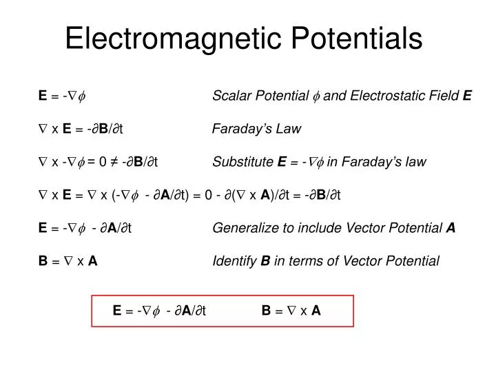
Electromagnetic Potentials. E = - f Scalar Potential f and Electrostatic Field E x E = - ∂ B / ∂ t Faraday’s Law x - f = 0 ≠ - ∂ B / ∂ t Substitute E = - f in Faraday’s law x E = x (- f - ∂ A / ∂ t) = 0 - ∂ ( x A )/ ∂ t = - ∂ B / ∂ t

E N D
Electromagnetic Potentials E= -fScalar Potential f and Electrostatic Field E x E = -∂B/∂t Faraday’s Law x -f = 0 ≠ -∂B/∂t Substitute E = -fin Faraday’s law x E = x (-f - ∂A/∂t) = 0 - ∂( x A)/∂t = -∂B/∂t E= -f - ∂A/∂t Generalize to include Vector Potential A B = x A Identify B in terms of Vector Potential E= -f - ∂A/∂t B = x A
Electromagnetic Potentials (A,f) 4-vector generates E, B 3-vectors ((A,f) redundant by one degree) Suppose (A,f) and (A’,f’) generate the same E, B fields E= -f - ∂A/∂t = -f’- ∂A’/∂t B = x A = x A’ Let A’ = A + f x A’ = x (A+ f) = x A+ x f = x A What change must be made to f to generate the same E field? E =-f’ - ∂A’/∂t = -f’ - ∂(A+ f)/∂t = -f - ∂A/∂t A’ = A + ff’= f- ∂f/∂t Gauge Transformation
Electromagnetic Potentials A = AL + AT L and T components of A A’ = AL + AT + f Change of gauge . A’ = . AL + . AT + . f = . AL+ 2 f . AT= 0 Choose . A’ = 0 f = -AL A’ = AT f’ = f - ∂f/∂t f’ = f- ∂f/∂t f’ = f+ ∂AL/∂t E = -f- ∂A/∂t = (-f) - ∂(AL+AT)/∂t x E = x (-f - ∂A/∂t) = x -∂AT/∂t x f= x ∂AL/∂t= 0 E = -f’- ∂A’/∂t = (-f - ∂AL/∂t) - (∂AT/∂t) x E = x -∂AT/∂t
Electromagnetic Potentials Coulomb Gauge Choose . A = 0 Represent Maxwell laws in terms of A,f potentials and j, r sources x B = moj + moeo∂E/∂t Maxwell-Ampère Law x ( x A) = moj + moeo∂(-f - ∂A/∂t)/∂t (. A)- A = moj – 1/c2 ∂f/∂t - 1/c2∂2A/∂t2 . E = r /eoGauss’ Law . (-f - ∂A/∂t) = -. f - ∂. A/∂t = - r /eo
Electromagnetic Potentials . A = 0 -2f = r /eoCoulomb or Transverse Gauge Coupled equations for A, f
Electromagnetic Potentials Lorentz Gauge Choose . A = – 1/c2∂f/∂t x B = moj + moeo∂E/∂t Maxwell-Ampère Law (. A)- A = moj – 1/c2 ∂f/∂t - 1/c2∂2A/∂t2 . E = r /eoGauss’ Law . (-f - ∂A/∂t) = -. f - ∂. A/∂t = -. f + 1/c2∂2f/∂t2 = r /eo
Electromagnetic Potentials . A= – 1/c2∂f/∂t Lorentz Gauge □2 □2 =
Electromagnetic Potentials □2 Each component of A, fobeys wave equation with a source □2 = □2G(r - r’, t - t’)= d(r - r’) d(t - t’) Defining relation for Green’s function d(r - r’) d(t - t’) Represents a point source in space and time G(r- r’, t - t’)= Proved by substitution ) is non-zero for i.e. time taken for signal to travel from r’ to r at speed c (retardation of the signal) ensures causality (no response if t’ > t)
Electromagnetic Potentials Solution in terms of G and source Let be the retardation time, then there is a contribution to from at t’ = t - . Hence we can write, more simply, c.f. GP Eqn 13.11 Similarly c.f. GP Eqn13.12 These are retarded vector and scalar potentials
Radiation by Hertz Electric Dipole r = (x, y, z) Field Point z +q Using retarded potentials, calculate E(r,t), B(r,t) for dipole at origin y l x r' = (0, 0, z’) Source Point -q Charge q(t) = qo Re {eiwt} Current I(t) = dq/dt = qoRe {iweiwt} Dipole Moment p(t) = poRe {eiwt} = qolRe {eiwt} Wire Radius a Current Density j(t) = I(t) / p a2
Radiation by Hertz Electric Dipole • Retarded Electric Vector Potential • A(r, t)A || ez because j || ez • Retardation time t = |r - ezz’| / c if l << c t then t≈ |r| / c = r / c • Az(r, t) for distances r >> l • . A = – 1/c2 ∂f/∂t Obtain f from Lorentz Gauge condition • . A= ∂Az(r, t) / ∂z = • = –∂f/∂t • ∂f/∂t =
Radiation by Hertz Electric Dipole • Differentiate wrt z and integrate wrtt to obtain • Az(r, t) • since d(t - r/c) = dt • Charge q(t) = qo Re {eiwt} • Current I(t) = = qoRe {iweiwt} Electric Field E(r, t) = - f -
Radiation by Hertz Electric Dipole • Switch to spherical polar coordinates • • - • k = w / c is the dipole amplitude
Radiation by Hertz Electric Dipole • Obtain part of E field due to A vector • Az(r, t) Cartesian representation • A(r, t) Spherical polar rep’n • - • - • -
Radiation by Hertz Electric Dipole • Total E field • E • Long range (radiated) electric field, proportional to • Erad • Radiated E field lines , polar plots
Radiation by Hertz Electric Dipole Short range, electrostatic field = 0 i.e. k = / c → 0 Total E field E Eelectrostat. = - Classic field of electric point dipole
Radiation by Hertz Electric Dipole • Obtain B field from x A • A(r, t) • Radiated part of B field • t)= / c
Radiation by Hertz Electric Dipole • Power emitted by Hertz Dipole • The Poynting vector, N, gives the flux of radiated energy Jm-2s-1 • The flux N = E x H depends on r and q, but the angle-integrated flux is constant • N = E x H = / mo
Radiation by Hertz Electric Dipole • = = > = • = • Average power over one cycle • = wqopo = qo po w =
Radiation by Half-wave Antenna Half Wave Antenna r = (x, y, z) Field Point z r’’ r q’ r' = (0, 0, z’) Source Point t – t – y q l/2 x Current distribution I(z’, t) = Iocos (2p z’/ l) eiwt Current distribution on wire is half wavelength and harmonic in time
Radiation by Half-wave Antenna • Single Hertz Dipole • = = / = • Current distribution in antenna (z’, t) = cos • Radiation from antenna is equivalent to sum of radiation from Hertz dipoles • t – t –
Radiation by Half-wave Antenna • Half Wave Antenna electric field • c.f. GP 13.24 NB phase difference • Hertz Dipole electric field • 1 • In general, for radiation in vacuum B = k x E / c, hence for antenna
Radiation by Half-wave Antenna • = • = • Average power over one cycle
Radiation by Half-wave Antenna • Half Wave Antenna • = • Polar plot for half wave antenna • Hertz Dipole • Polar plot for Hertz dipole