Download
1 / 35
360 likes | 415 Views
Discover the advancements in frequent pattern mining for streaming data and ways to approximate frequent patterns with good accuracy. Learn about the Lossy Counting Algorithm, space-saving computation methods, and mining evolution of patterns over time.

E N D
Frequent Patterns for Stream Data • Frequent pattern mining is valuable in stream applications • e.g., network intrusion mining (Dokas, et al’02) • Mining precise freq. patterns in stream data: unrealistic • Even store them in a compressed form, such as FPtree • How to mine frequent patterns with good approximation? • Approximate frequent patterns (Manku & Motwani VLDB’02) • Keep only current frequent patterns? No changes can be detected • Mining evolution freq. patterns (C. Giannella, J. Han, X. Yan, P.S. Yu, 2003) • Use tilted time window frame • Mining evolution and dramatic changes of frequent patterns • Space-saving computation of frequent and top-k elements (Metwally, Agrawal, and El Abbadi, ICDT'05)
Mining Approximate Frequent Patterns • Mining precise freq. patterns in stream data: unrealistic • Even store them in a compressed form, such as FPtree • Approximate answers are often sufficient (e.g., trend/pattern analysis) • Example: a router is interested in all flows: • whose frequency is at least 1% (σ) of the entire traffic stream seen so far • and feels that 1/10 of σ (ε= 0.1%) error is comfortable • How to mine frequent patterns with good approximation? • Lossy Counting Algorithm (Manku & Motwani, VLDB’02) • Major ideas: not tracing items until it becomes frequent • Adv: guaranteed error bound • Disadv: keep a large set of traces
Bucket 1 Bucket 2 Bucket 3 Lossy Counting for Frequent Items Divide Stream into ‘Buckets’ (bucket size is 1/ ε = 1000)
Empty (summary) + At bucket boundary, decrease all counters by 1 First Bucket of Stream
+ At bucket boundary, decrease all counters by 1 Next Bucket of Stream
Approximation Guarantee • Given: (1) support threshold: σ, (2) error threshold: ε, and (3) stream length N • Output: items with frequency counts exceeding (σ–ε) N • How much do we undercount? If stream length seen so far = N and bucket-size = 1/ε then frequency count error #buckets = εN • Approximation guarantee • No false negatives • False positives have true frequency count at least (σ–ε)N • Frequency count underestimated by at most εN
Bucket 1 Bucket 2 Bucket 3 Lossy Counting For Frequent Itemsets Divide Stream into ‘Buckets’ as for frequent items But fill as many buckets as possible in main memory one time If we put 3 buckets of data into main memory one time, Then decrease each frequency count by 3
2 2 4 3 1 4 3 2 10 1 2 + 9 1 2 1 0 3 bucket data in memory summary data Update of Summary Data Structure summary data Itemset ( ) is deleted.That’s why we choose a large number of buckets – delete more
1 2 Pruning Itemsets – Apriori Rule 2 + 1 1 3 bucket data in memory summary data If we find itemset ( ) is not frequent itemset, Then we needn’t consider its superset
Summary of Lossy Counting • Strength • A simple idea • Can be extended to frequent itemsets • Weakness: • Space Bound is not good • For frequent itemsets, they do scan each record many times • The output is based on all previous data. But sometimes, we are only interested in recent data • A space-saving method for stream frequent item mining • Metwally, Agrawal and El Abbadi, ICDT'05
Mining Evolution of Frequent Patterns for Stream Data • Approximate frequent patterns (Manku & Motwani VLDB’02) • Keep only current frequent patterns—No changes can be detected • Mining evolution and dramatic changes of frequent patterns (Giannella, Han, Yan, Yu, 2003) • Use tilted time window frame • Use compressed form to store significant (approximate) frequent patterns and their time-dependent traces • Note: To mine precise counts, one has to trace/keep a fixed (and small) set of items
Two Structures for Mining Frequent Patterns with Tilted-Time Window • FP-Trees store Frequent Patterns, rather than Transactions • Tilted-time major: An FP-tree for each tilted time frame
Frequent Pattern & Tilted-Time Window (2) • The second data structure: • Observation: FP-Trees of different time units are similar • Pattern-tree major: each node is associated with a tilted-time window
Classification for Dynamic Data Streams • Decision tree induction for stream data classification • VFDT (Very Fast Decision Tree)/CVFDT (Domingos, Hulten, Spencer, KDD00/KDD01) • Is decision-tree good for modeling fast changing data, e.g., stock market analysis? • Other stream classification methods • Instead of decision-trees, consider other models • Naïve Bayesian • Ensemble (Wang, Fan, Yu, Han. KDD’03) • K-nearest neighbors (Aggarwal, Han, Wang, Yu. KDD’04) • Tilted time framework, incremental updating, dynamic maintenance, and model construction • Comparing of models to find changes
Hoeffding Tree • With high probability, classifies tuples the same • Only uses small sample • Based on Hoeffding Bound principle • Hoeffding Bound (Additive Chernoff Bound) r: random variable R: range of r n: # independent observations Mean of r is at least ravg – ε, with probability 1 – d
Hoeffding Tree Algorithm • Hoeffding Tree Input S: sequence of examples X: attributes G( ): evaluation function d: desired accuracy • Hoeffding Tree Algorithm for each example in S retrieve G(Xa) and G(Xb) //two highest G(Xi) if ( G(Xa) – G(Xb) > ε ) split on Xa recurse to next node break
Decision-Tree Induction with Data Streams Packets > 10 Data Stream yes no Protocol = http Packets > 10 Data Stream yes no Bytes > 60K Protocol = http yes Ack. From Gehrke’s SIGMOD tutorial slides Protocol = ftp
Hoeffding Tree: Strengths and Weaknesses • Strengths • Scales better than traditional methods • Sublinear with sampling • Very small memory utilization • Incremental • Make class predictions in parallel • New examples are added as they come • Weakness • Could spend a lot of time with ties • Memory used with tree expansion • Number of candidate attributes
VFDT (Very Fast Decision Tree) • Modifications to Hoeffding Tree • Near-ties broken more aggressively • G computed every nmin • Deactivates certain leaves to save memory • Poor attributes dropped • Initialize with traditional learner (helps learning curve) • Compare to Hoeffding Tree: Better time and memory • Compare to traditional decision tree • Similar accuracy • Better runtime with 1.61 million examples • 21 minutes for VFDT • 24 hours for C4.5 • Still does not handle concept drift
CVFDT (Concept-adapting VFDT) • Concept Drift • Time-changing data streams • Incorporate new and eliminate old • CVFDT • Increments count with new example • Decrement old example • Sliding window • Nodes assigned monotonically increasing IDs • Grows alternate subtrees • When alternate more accurate => replace old • O(w) better runtime than VFDT-window
Ensemble of Classifiers Algorithm • H. Wang, W. Fan, P. S. Yu, and J. Han, “Mining Concept-Drifting Data Streams using Ensemble Classifiers”, KDD'03. • Method (derived from the ensemble idea in classification) • train K classifiers from K chunks • for each subsequent chunk train a new classifier test other classifiers against the chunk assign weight to each classifier select top K classifiers
Clustering Data Streams [GMMO01] • Base on the k-median method • Data stream points from metric space • Find k clusters in the stream s.t. the sum of distances from data points to their closest center is minimized • Constant factor approximation algorithm • In small space, a simple two step algorithm: • For each set of M records, Si, find O(k) centers in S1, …, Sl • Local clustering: Assign each point in Si to its closest center • Let S’ be centers for S1, …, Sl with each center weighted by number of points assigned to it • Cluster S’ to find k centers
Hierarchical Clustering Tree level-(i+1) medians level-i medians data points
Hierarchical Tree and Drawbacks • Method: • maintain at most m level-i medians • On seeing m of them, generate O(k) level-(i+1) medians of weight equal to the sum of the weights of the intermediate medians assigned to them • Drawbacks: • Low quality for evolving data streams (register only k centers) • Limited functionality in discovering and exploring clusters over different portions of the stream over time
Clustering for Mining Stream Dynamics • Network intrusion detection: one example • Detect bursts of activities or abrupt changes in real time—by on-line clustering • Our methodology (C. Agarwal, J. Han, J. Wang, P.S. Yu, VLDB’03) • Tilted time frame work: o.w. dynamic changes cannot be found • Micro-clustering: better quality than k-means/k-median • incremental, online processing and maintenance) • Two stages: micro-clustering and macro-clustering • With limited “overhead” to achieve high efficiency, scalability, quality of results and power of evolution/change detection
CluStream: A Framework for Clustering Evolving Data Streams • Design goal • High quality for clustering evolving data streams with greater functionality • While keep the stream mining requirement in mind • One-pass over the original stream data • Limited space usage and high efficiency • CluStream: A framework for clustering evolving data streams • Divide the clustering process into online and offline components • Online component: periodically stores summary statistics about the stream data • Offline component: answers various user questions based on the stored summary statistics
The CluStream Framework • Micro-cluster • Statistical information about data locality • Temporal extension of the cluster-feature vector • Multi-dimensional points with time stamps • Each point contains d dimensions, i.e., • A micro-cluster for n points is defined as a (2.d + 3) tuple • Pyramidal time frame • Decide at what moments the snapshots of the statistical information are stored away on disk
CluStream: Pyramidal Time Frame • Pyramidal time frame • Snapshots of a set of micro-clusters are stored following the pyramidal pattern • They are stored at differing levels of granularity depending on the recency • Snapshots are classified into different orders varying from 1 to log(T) • The i-th order snapshots occur at intervals of αi where α≥ 1 • Only the last (α + 1) snapshots are stored
CluStream: Clustering On-line Streams • Online micro-cluster maintenance • Initial creation of q micro-clusters • q is usually significantly larger than the number of natural clusters • Online incremental update of micro-clusters • If new point is within max-boundary, insert into the micro-cluster • O.w., create a new cluster • May delete obsolete micro-cluster or merge two closest ones • Query-based macro-clustering • Based on a user-specified time-horizon h and the number of macro-clusters K, compute macroclusters using the k-means algorithm
Stream Data Mining: Research Issues • Mining sequential patterns in data streams • Mining partial periodicity in data streams • Mining notable gradients in data streams • Mining outliers and unusual patterns in data streams • Stream clustering • Multi-dimensional clustering analysis? • Cluster not confined to 2-D metric space, how to incorporate other features, especially non-numerical properties • Stream clustering with other clustering approaches? • Constraint-based cluster analysis with data streams?
Summary: Stream Data Mining • Stream data mining: A rich and on-going research field • Current research focus in database community: • DSMS system architecture, continuous query processing, supporting mechanisms • Stream data mining and stream OLAP analysis • Powerful tools for finding general and unusual patterns • Effectiveness, efficiency and scalability: lots of open problems • Our philosophy on stream data analysis and mining • A multi-dimensional stream analysis framework • Time is a special dimension: Tilted time frame • What to compute and what to save?—Critical layers • partial materialization and precomputation • Mining dynamics of stream data