Download
1 / 19
270 likes | 1.02k Views
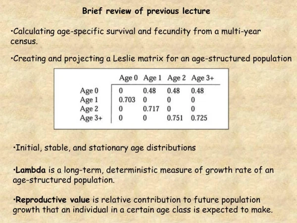
Age-structured models (continued): Estimating l from Leslie matrix models. Fish 458, Lecture 4. The facts on l. Finite rate of population increase l =e r & r=ln( l ), therefore N t =N l t A dimensionless number (no units) Associated with a particular time step

E N D
Age-structured models (continued):Estimating l from Leslie matrix models Fish 458, Lecture 4
The facts on l • Finite rate of population increase • l=er & r=ln(l), therefore Nt=Nlt • A dimensionless number (no units) • Associated with a particular time step • (Ex: l =1.2/yr not the same as l = 0.1/mo) • l >1: pop. ; l<1 pop
Matrix Population Models: Definitions • Matrix- any rectangular array of symbols. When used to describe population change, they are called population projection matrices. • Scalar- a number; a 1 X 1 matrix • State variables- age or stage classes that define a matrix. • State vector- non-matrix representation of individuals in age/stage classes. • Projection interval- unit of time define by age/stage class width.
Basic Matrix Multiplication 4x1 + 3x2 + 2x3= 0 2x1 - 2x2 + 5x3= 6 x1 - x2 - 3x3= 1 x1 x2 x3 0 6 1 4 3 2 2 –2 5 1 –1 3 =
What does this remind you of? n(t + 1) = An(t) Where: Ais the transition/projection matrix n(t) is the state vector n(t + 1) is the population at time t + 1 This is the basic equation of a matrix population model.
Eigenvectors & Eigenvalues When matrix multiplication equals scalar multiplication vA = v Aw = w v,w = Eigenvector = Eigenvalue • Rate of Population Growth (): Dominant Eigenvalue • Stable age distribution (w): Right Eigenvector • Reproductive values (v): Left Eigenvector Note: “Eigen” is German for “self”.
Example: Eigenvalue Ax = y Ax = y • -6 • 2 -5 4 1 6 3 • -6 • 2 -5 1 1 -3 -3 = = No obvious relationship between x and y Obvious relationship between x and y:x is multiplied by -3 Thus, A acts like a scalar multiplier. How is this similar to ?
Characteristic equations From eigenvalues, we understand thatAx = x We want to solve for , so Ax - x = 0 (singularity) or (A- I)x = 0 “I”represents an identity matrix that converts into a matrix on the same order as A. Finding the determinant of (A- I) will allow one to solve for . The equation used to solve for is called the Characteristic Equation
Solution of the Projection Equationn(t+1)=An(t) 4 - P1F2 2 - P1P2F3 - P1P2P3F4 = 0 or alternatively (divide by 4) 1 = P1F2 -2 + P1P2F3 -3 + P1P2P3F4 -4 This equation is just the matrix form of Euler’s equation: 1 = Σlxmxe-rx
Constructing an age-structured (Leslie) matrix model • Build a life table • Birth-flow vs. birth pulse • Pre-breeding vs. post-breeding census • Survivorship • Fertility • Build a transition matrix
Birth-Flow vs. Birth-Pulse • Birth-Flow (e.g humans)Pattern of reproduction assuming continuous births. There must be approximations to l(x) and m(x); modeled as continuous, but entries in the projection matrix are discrete coefficients. • Birth-Pulse (many mammals, birds, fish)Maternity function and age distribution are discontinuous, matrix projection matrix very appropriate.
Pre-breeding vs. Post-breeding Censuses Pre-breeding (P1) Populations are accounted for just before they breed. Post-breeding (P0) Populations are accounted for just after they breed
Calculating Survivorship and Fertility Rates for Pre- and Post-Breeding Censuses Different approaches, yet both ways produce a of 1.221.
The Transition/Population Projection Matrix 4 age class life cycle graph
Example:Shortfin Mako (Isurus oxyrinchus) Software of choice: PopTools
Mako Shark Data Mortality: M1-6 = 0.17 M7-w = 0.15 Fecundity: 12.5 pups/female Age at female maturity: 7 years Reproductive cycle: every other 2 years Photo: Ron White
Essential Characters of Population Models • Asymptotic analysis: A model thatdescribes the long-term behavior of a population. • Ergodicity: A model whose asymptotic analyses are independent of initial conditions. • Transient analysis: The short-term behavior of a population; useful in perturbation analysis. • Perturbation (Sensitivity) analysis: The extent to which the population is sensitive to changes in the model. Caswell 2001, pg. 18
Uncertainty and hypothesis testing • Characterizing uncertainty • Series approximation (“delta method”) • Bootstrapping and Jackknifing • Monte Carlo methods • Hypothesis testing • Loglinear analysis of transition matrices • Randomization/permutation tests Caswell 2001, Ch. 12
References Caswell, H. 2001. Matrix Population Models: Construction, Analysis, and Interpretation. Sunderland, MA, Sinauer Associates. 722 pp. Ebert, T. A. 1999. Plant and Animal Populations: Methods in Demography. San Diego, CA, Academic Press. 312 pp. Leslie, P. H. 1945. On the use of matrices in certain population mathematics. Biometrika 33: 183-212. Mollet, H. F. and G. M. Cailliet. 2002. Comparative population demography of elasmobranch using life history tables, Leslie matrixes and stage-based models. Marine and Freshwater Research 53: 503-516. PopTools: http://www.cse.csiro.au/poptools/